Understanding Distortion: A Look At Electronics

A Look At Distortion Mechanisms

Built With Purpose

In writing this article, the mission has been to demonstrate and explain several types of distortion which are exhibited among electronic audio devices. You will not find any extensive differential equations, nor three-space analysis here. Instead, the didactic has been to provide a practical and predominantly layman’s terms paper, to explain more to the listener about what distortion is and what else engineers look for when designing audio equipment. Beginning at nearly one-hundred pages total and being exclusively based on years in electronics design, this article has been edited down to a more casual two-part article.

Built on a foundation of verisimilitude, the prime purpose has been to shed some light on why any number of sources, pre-amplifiers, or power amplifiers may appear identical based on their brochures’ depicted performance, and yet sound quite different from one another. The goal has also been to avoid being perfunctory, while offering an informative set of explanations for a variety of key terms that may have otherwise left readers unsure of their true meanings. To supplement the descriptions, several images have been produced that depict distortions as they occur. With this acknowledgement in hand, it is my hope that readers may gain an enlightened understanding of what distortion is, and how it affects audio reproduction.

Firstly, What Is Audio?

We love music and sound, and in our efforts to describe sonic events in ways that they can be related and repeated, we have assigned mathematical conditions and terminology to make them easier to understand. As readers, we all have possibly been exposed to the repeated mentions of specific terminology. Among them, readers may recall discussions centered around the topic of waveforms. What are waveforms, you may ask? Waveforms serve as universal descriptors for an event that has both a geomatic magnitude (ie: level, relative intensity) and progressive direction in relative time. What that means, is that waveforms represent an intensity, level, or pneumatic pressure that changes as time passes.

In the physical realm of audio, waveforms are used to share information about the variances in air pressure and the kinetic motion of a sound-generating medium. Examples of sources of physical and acoustic stimulus include vibrating membranes, such as loudspeakers’ diaphragms enacting an oscillation upon the surrounding air mass. The high and low pressure oscillations in air pressure eventually reach our ears, a microphone, a surface that an accelerometer has been mounted to, or the surface plane adjacent to a laser spectrometer which also reacts to the acoustic propagation. Each of these situations entail a mechanism by which they can understand the waveform. However, in a vacuum there may be an initial source of motion, but there can be no sound in a space without a gaseous, liquid, or solid state of matter to permit the transfer of physical and acoustical energy.

Most sounds are comprised of numerous sinuous pulses and oscillations, as the result of compressions and rarefactions of the air molecules. Others sounds are formed with the addition of sharper shaped crests, or edges, and any may be present as beats, modes, or pseudo-random spurious transients. In the beginning, the initial pulses of sounds begin as a climbing pressure. The tympanic membrane of the ear (eardrum) moves inward in direct response to this increase in pressure. The air pressure eventually ceases to climb and recedes, dropping in pressure and causing the tympanic membrane to moved back to its resting position. If the sound is not just an impulse and is ongoing, the pressure alternates between positive, neutral, and negative coefficients, and the tympanic membrane continues to move inward and outward in a similar fashion. Each complete waveform cycle takes place within the course of 360 degrees, and cycles can also continue for extended periods, if not indefinitely.

A vast increase in positive and negative pressure, that is to say intensity, impinges upon the ear’s typmanic membrane, causing it to move more and thus increasing the level of intensity. The term Magnitude is used to describe the intensity and level of any specific event, or factor, and in most instances it directly relates to perceived loudness, represented by unit measurement system of Decibels. Decibels are derived from the term Bel, a logarithmic unit of measurement with a base value of 10, with one Bel being equal to ten decibels. For the purpose of this paper, the term decibel will be the prime descriptor for relative magnitude of loudness.

In the realm of electronics engineering & audio design, waveforms and sine waves also form a means of universally representing the alternating nature of voltage and current. Just like acoustic phenomenon, the analog electric interpretation is based on geomatic magnitude versus time. Much like acoustic pressure, electrical waveforms can be very complex and formed on many different sinuous and spurious signals, combining additive and subtractive attributes.

The Nature Of Waveforms. Please Click On Image To Enlarge

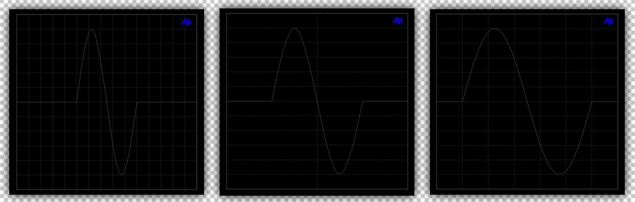
In the Figure above, we see common sinuous cycles. The first image of a waveform on the left side has been labelled to show four quadrants; 0-90 degrees; 90-180 degrees; 180-270 degrees; and 270-360 degrees. The initial stage climbs from 0 to 90 degrees as it rises from zero potential to the peak value. What goes up must come down, and the fall in magnitude from 90 to 180 degrees brings the sine wave back to zero potential through rarefaction. This is one pulse, and constitutes a half cycle. For it to form a sinuous cycle, it must complete a full 360 degrees. Following the waveform, it progresses from 180 degrees to 270, forming the full negative peak. The difference in potential between the 90 to 270 degree points forms the basis of a peak-to-peak magnitude. The signal then traverses 270 to 360 degrees, once again making its way to zero potential. Every sinuous frequency makes this same journey, and as mentioned earlier it can be ongoing.

The center Figure  in the above image depicts the same magnitude and frequency, but with an opposite phase, or polarity. Phase and polarity are not one and the same, but within this context they are interchangeable. Notice that it looks just like the sine wave in Figure 1, except that it is upside down. This waveform occurs with an identical starting point, the same magnitude, and even traverses the zero potential point of alteration and ends in the same relative time. The difference is, that this one begins at 180 degrees instead of 0. This is what we refer to as being 180 degrees out of phase. That is pretty simple, isn’t it? Many electronics reverse the phase of an incoming signal as a function of how they are designed and operate. A single electronic gain stage using feedback will alter the final output signal phase by 180 degrees. Two stages set the output at 360 degrees, which is considered to be phase correct. In this way, two consecutive stages will retain the integrity of the original phase, and is what is refer to as Absolute Phasing.

The last Figure on the far right side is an example of amplification, where in this case the smaller inset signal is increased in magnitude by a factor of four times. The signal maintains the same time span and thus the same frequency. Although the human ocular perception of the figure’s shape  may be confusing, it retains the same sinuous curve contour and it is only larger. The foremost goal of amplification is to increase the level of a signal, be it a lone waveform, the complex sum of several, or one of musical nature.

20kHz, 1kHz, and 20Hz Sine Waves. Please Click On Image To Enlarge.

It is interesting that the number of pressure variations within a given time span determine the perceived pitch, or tone. We use the term frequency, represented as Hertz (Hz) to explain the relationship between a complete cycle versus time. Above, the Figure displays three frequencies.  The first one the left is a single cycle with a time stamp corresponding to 20,000 cycles per second (20kHz), and this single cycle covers a relatively short duration of 50 microseconds. The second is a single cycle corresponding to a frequency of 1000 cycles per passing second (1kHz), which always takes place over 1 millisecond. Thirdly, the final is 20 cycles per second (20Hz) and last for 50 milliseconds. All are at the same peak voltage magnitude, and share the exact identical waveform shape. As demonstrated by these graphs, we can understand that modifying the length of time it takes for each cycle to complete directly changes the frequency and perceived pitch.

While some may consider the aspects of human hearing to be a benchmark, our hearing is far from linear. The auditory system’s frequency response to acoustic stimulus is non-linear in nature, meaning that it is not consistent and does not follow a straight line. The response to high and low frequencies attenuates outside of a narrow plateau that is typically formed by two resonance nodes. For most listeners, the location of these nodes, which happen to constitute the most sensitive portion of the hearing spectrum, reside between 2000 cycles per each passing second (2kHz) to 4000 cycles (4kHz) per second. The commonly accepted full bandwidth resides between 20Hz and 20kHz, and narrows with age, health status, and noise exposure.

We do not perceive loudness in a linear manner. Rather, our hearing is logarithmic. This is known as the Weber-Fechner Law, and applies to all our senses. What this means is that a change in acoustic power of ten times results in a perceived loudness of only two times. The perception of loudness is also affected by the quantity of variations of sounds within a given time frame, and duration of the stimulus, known as Sones. Hearing threshold is another factor in hearing, and varies from one individual to another with age and exposure to noise. Threshold is the sensitivity to the quietest sounds, and below this point sounds cannot be heard, nor distinguished from the mechanics of the body.

At this stage we have established that humans hear pitch, do not perceive loudness in a linear manner, and that there is a limit to how quiet sounds can be heard. To make matters even more complex, the auditory system does not receive tones and pitch as a linear function of frequency shift, either. Instead, this aspect of auditory response is pre-cortical. The frequency range can be divided into Decades of  0-100 cycles, 100-1k cycles, 1k-10k cycles and 10k-100k cycles. Once over, the commonly claused hearing range is approximately 20 Hertz to 20k cycles, but as the frequency is increased within a Decade, the perceived change in pitch becomes dramatically reduced. More descriptive of this phenomenon, a change in pitch between 1000 Hertz and 1010 Hertz is audible, and there is a lot of information to be had between 1kHz and 2kHz. However, a change from 9000 Hertz to 9010 Hertz is much more difficult to identify, as moving from 9000 Hertz to 10,000 is a perceived as a brief event, indeed. Another example would be how easily a subject can hear, or otherwise sense a shift from 20Hz to 23Hz which belies the lower end of the lowest decade. Meanwhile, a shift from 90Hz to 93Hz is perceived as much smaller, despite still being the same difference of 3Hz.

Our perception of sound is very complex, and so is audio reproduction. Now that we have covered a little about what sound is, the primary topic of distortion should come as a bit easier to follow.

Distortion In The Electronic Age

Currently, imperfection appears to be a relative part of everything around us. Being imperfect devices, all electronics alter a signal passing through them, often in a variety of different ways and to varying extents. No amplifier or electronic device is exempt from this fact of life, although some are better at their tasks than others. Sometimes, these secondary emissions are injected upon the signal, bringing with them a great cumulative effect upon the accuracy of reproduction of the waveforms. Any modifications and changes, be them linear or non-linear in classification, large or small, are categorized as distortion. In that way, a signal is distorted when it is somehow different than it originally was.

Every signal builds upon the fundamental building block of audio – the sinusoidal waveform, as was previously discussed. From that essential starting point, any known signal could be derived. Be it square, triangle, sawtooth, quarter-wave partials, half-wave, lined with a variety of harmonic and inharmonic additions, beats and modulated subtractives, they all begin with the same starting point. It is with the addition of these factors that waveforms make the move away from being sinuous to becoming the complex sounds and signals we use and hear everyday.

Outside of electronics, there is a third z-designated tuple; in other words, a third dimension and point of direction, one that forms the natural acoustic phenomenon. However, all audio within the electronic domain operates in a two-dimensional manner. The voltage and/or current increase and decrease over time to recreate sound waveforms based a microphone’s single capture point. Understanding that electronic audio signals are comprised of a geomatic magnitude versus a direction in relative time, it then becomes much easier to relate to the facts comprising distortion in the electronic age.

Within the scope of electronics design, the longstanding collective goal of high fidelity has been to reduce unwanted distortions to such levels that they are indistinguishable from the important original waveforms. As a result, countless topologies and technologies have found there way into various examples of audio equipment. A secondary goal has also emerged; one that has been to manipulate distortion artifacts to tailor the sound of a product to a set of other design principles. This has posed many challenges for scientists & specialized engineers in the field of audio reproduction, but great progress has been made.

Having been designing electronics for a good portion of my own life, I was afforded the good fortune of being able to design some of my own analyzers and logic processors, as needed. Through the use of such tools and experience,  various aspects of sound and electrical behaviors were uncovered, and different forms of distortion modulus were then classified. Working with a number of research professors, we had striven to isolate various characteristics of sounds that provoked repeatable responses from listening subjects. Tests involved altering signals to help identify what was acceptable and what was not. With their assistance, and that of a K. Gordon of NASA, empirical factors were derived & assigned to imaging strength and the common term of sound-stage. Most of these are explained with the Head-Related Transfer Function (HRTF).

The head-related transfer function describes the frequency response, phase and impulse behaviors as sound reaches the listening subject’s ears. Dolby Laboratories (headed by Mark F. Davis) and the Fraunhofer Institute were among the largest organizations involved in this research. It was determined that both of those aforementioned temporal contexts – imaging and soundstage – originated within the auditory system’s neural processing, not the ears. We were aware of a series of invaluable acoustic parameters to measure, as they modified these attributes to good effect. The research leading to this has stemmed from the study of binaural sources, the shape of the ear and physical modeling. What was learned correlated closely with the theoretical; that when sound strikes the lobs and enters the canal from various angles, it superimposed a change in phase, frequency de-emphasis, and thus altered apparent waveform shape.

Today, the results of research can be realized firsthand through listening to any variety of high performance audio and home theater systems, and even more affordable sound bars strictly making use of forward channels only. Some could convincingly impose an impression upon the listeners that there were additional radiating planes aft of their seated positions. Other examples of acoustic perception modeling were used in the development of multi-channel encoding. A two channel audio stream containing three or more additional channels remains undetectable in conventional playback. This was distortion research being put to viable use, and it helped to build a better sounding amplifier and speaker system.

Data Capture and Presentation Compliance

This new age has seen many great and wondrous things, and among them, technology has progressively become more accessible. Such circumstances have also paved way for lower cost substitutions in essentially every sector. What used to be expensive to manufacture can now be done quickly and often efficiently. This has also introduced a variety of new problems, and measurement equipment has not been exemplified, nor immune to this trend. The proliferation of low-quality universal serial bus (USB) based testing hardware and associated software have been plaguing industries at an accelerate rate. As a result, quality control engineering specialists and consultants have been actively routing out the sources of non-compliance.

Most of the problem has been the result of third-party open-source software and improperly designed hardware. As a result of the low investment required, buyers of whom are unaware of the immediate differences are attracted to the low initial costs. Such devices make use of overzealous filtering, under-filtering, insufficient sampling rates, and mixed interpolation. Making things more difficult, the isolation of critical hardware components and the calibration of such systems is often non-existent or very conditional, as are the results.

For virtually all, the stimulus is captured via the device and sensors, then data points are created and interpreted by third-party software, while the calculations are carried by personal computers which have not been optimized. It is common that these devices only perform at a specific level and bandwidth, and that they fail to filter the fundamentals and make attempts to measure below their own noise flow through the use of active dithering. Like a three-hundred dollar automobile paint job, corners have been cut to meet their target price point.

Another concerning situation being readily faced today is the lack of the proper introduction and user training. In much the same way that young drivers have to become acquainted with the rules of the roads and how an automobile drives, familiarity and procedures are also pertinent when employing sophisticated (as well as simpler types of) measurement systems. It is important for the tester to identify that the results of a test are dependent upon utilizing the system as the designers intended. Outside factors can have profound impacts upon empiricism.  In short, the user must be familiarized with scientific testing methodology. Scientific method forms the foundation for unbiased qualification and quantification. We do not know everything about sound, and maybe never will.  We can only use science to help us understand acoustic phenomenon and how we interpret it. In other words, it’s purpose is to permit natural and controlled reactions and interactions to find a result that is true and repeatable.

Laboratory equipment, like those which are available from many qualified providers, such as Hewlett Packard, Audio Precision, Brüel & Kjær, and R&S among others. That equipment bases itself on the extensive testing, consideration and documentation of parasitic factors, and the adoption of intuitive & proprietary design principles. In short, a better and more reliable degree of accuracy. High-grade equipment features most, if not all, the measurement capture hardware and software inclusive to a closed network, and this helps greatly. Among the benefits of such systems comes ease of use, shielding from noise, freedom from interface mismatching, and calibration issues. In this way, they can offer the utmost reliable extrapolation and representation of the test data.

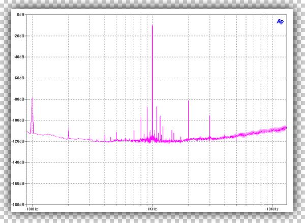
The results can be viewed on the machine’s own screen, along with an associated computer if the user wishes to export the results for third-party review. In this way, the testing equipment does the heavy lifting internally so that a personal computing device becomes an accessory that simply permits sharing of the data. In the past, some measurements could only be shared via photographs of, for example, Hewlett Packard oscilloscopes and analyzer screens. Whilst perhaps not as pleasing to the modern eye, these systems were a part of the reliable foothold of engineering and design. I will apologize for my own images that are greatly reduced in size. A reader can actively identify reliable presentations of forthcoming data by looking for the respected “Ap” and “Brüel & Kjær” trademarks, among others found on the upper right-hand corners of test results, and by inquiring with the professionals to whom the device(s) are licensed to.

The goal of this article is that the reader may gain a better understanding of what distortion in audio electronics is, and that one or two simple measurements may be non-descriptive of the more complex behaviors. Following the link below, we will take a look and not sweat the minutia.

Article continues:

Understanding Distortion: A Look At Electronics, Part 2