
A Look At Distortion Mechanisms
This paper is continued from the introduction to Understanding Distortion: A Look At Electronics.
Harmonic Distortion
Harmonic Distortion is a non-linear behavior occurring not only within the world of electronics, but among acoustic phenomenon as well. This behavior is characterized by multiples of the input signal(s) which were not present in the original input waveform. Commonly abbreviated as H.D, a harmonic is an additional signal whose frequency is an integral whole-number multiple of the frequency of a fundamental (input) reference signal.
Harmonics can be even and odd ordered, and often cover a wide upward bandwidth. For a signal whose fundamental frequency is referenced as f1, the second harmonic would have a frequency twice as high, ie: two times f1. A third harmonic would have a frequency three times as high as f1, and so on. This can be demonstrated by starting with a signal of 1000 cycles per passing second (1kHz). The second and third harmonics for this fundamental would be 2kHz and 3kHz. If the signal is complex and comprised of a multitude of fundamentals, there can also be harmonics for each and every one. Higher even-orders of harmonics include 4th, 6th, and 8th harmonics, and higher odd-orders include 5th, 7th, and 9th harmonics.
As the harmonic spectrum becomes richer with new harmonics, the waveform takes on a more complex appearance, indicating greater deviation from the ideal original one. A closely sorted and high-level harmonic spectrum may completely obscure the intended input signal. In the case of such input being sinusoidal, it can effectively distort the signal, thereby making the waveform unrecognizable. In this way, it would be important to control, if not minimize the relative intensity of such distortions.
In the consumerist electronics industry, it is rare to see Harmonic Distortion presented in a manner that individually identifies each harmonic. The standardized measure for distortion in electronics is Total Harmonic Distortion, which uses a single numerical expression based on steady-state sinuous waveform signals in accordance with IHF standards. Often abbreviated as T.H.D, it is the summed total of all relevant harmonics then expressed as a logarithmic percentage of the total signal magnitude. While the harmonic spectra holds great importance during design, T.H.D provides a quick reference to the maximum levels of harmonic distortion. The T.H.D rating of a power amplifier, or other device, refers to the creation of unwanted harmonics by the device during it’s intended and most linear mode of operation.
Second and third-order harmonic distortions are the most common types naturally occurring in stages of signal amplification. They are also typically the highest in magnitude. This holds true for both solid-state and hollow-state technologies, and they reside among the most easily modeled forms of non-linear behavior. The supporting circuitry within a stage of amplification can be tailored to reduce, enhance, or modify the sequential orders of harmonic distortion, with second-order harmonics being the easiest to reduce to vanishingly low levels.
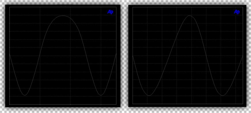
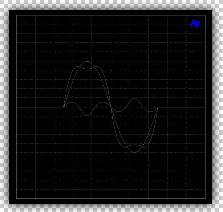
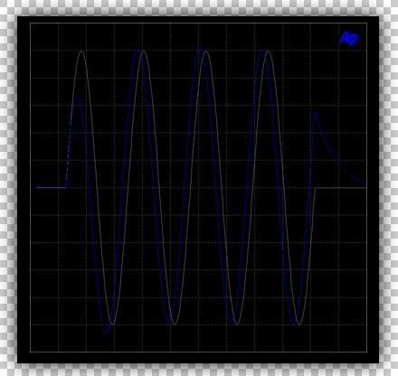
Depending on the phase of a second-order harmonic, it can impose varying effects on the original signal. Should the harmonic be in phase, it can tilt the waveform by sharpening the positive 0-90 degree and 180-270 degree slopes while flattening the points at 90-180 degrees and 270-360 degrees of each cycle. If the harmonic is out of phase with the signal, it can produce tilted waveform in the opposed fashion. If the harmonic is 90 degrees out of phase it can cause one half to becomes rounded while the other is sharpened, as depicted in the first Figure above. These are very different effects which have received very little discussion in the public eye.
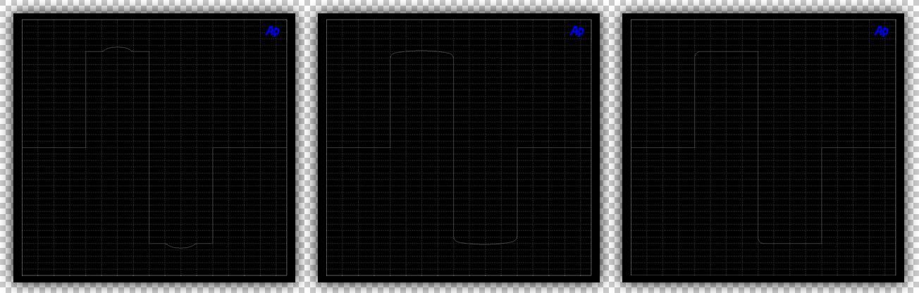
For several decades, it has been more or less accepted that second order may be the most tolerable distortion to the human auditory system. Recent years have brought the concept of even ordered harmonics being perceived as better sounding into question. Along with this past belief was one that solid-state devices produced the most pronounced spectrum of high-order harmonic content. Measurements validate that such claims are mistaken, and quite contrary. The de facto remains that hollow-state typically produces the highest levels of high-order content, both even and odd-ordered. If the goal is low or tailored harmonic distortion, it is very attainable. What is important, if that that third-order harmonics are now being looked at in a different light. Under certain conditions, they can been interpreted as equally acceptable in listening, and sometimes even more so. In addition, nearly all carbon fiber loudspeaker drive units, electrostatic loudspeakers, and many tetrode & pentode amplifiers exhibit predominantly third ordered harmonics. Let’s take a few moments to investigate this order of harmonics further.
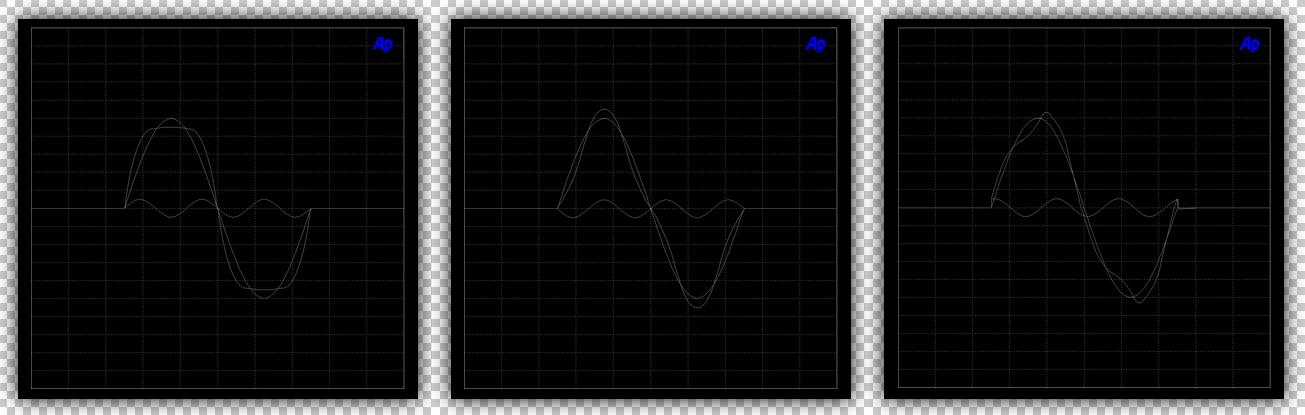
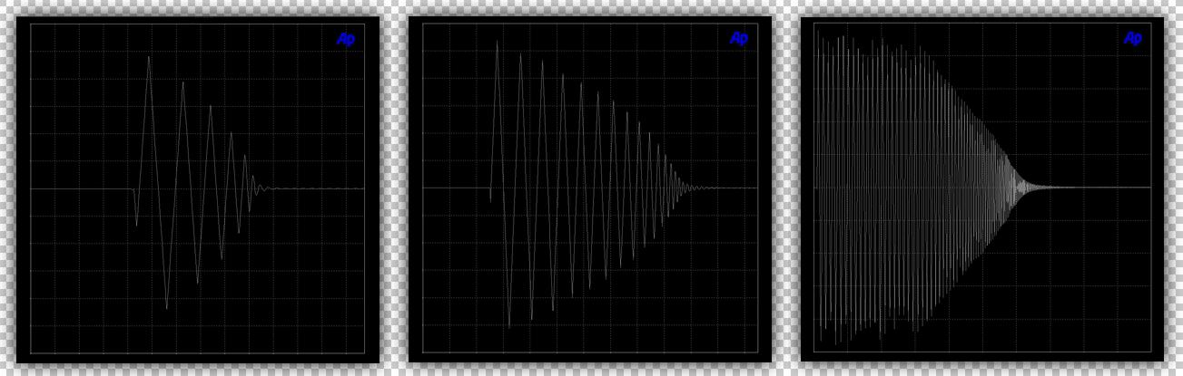
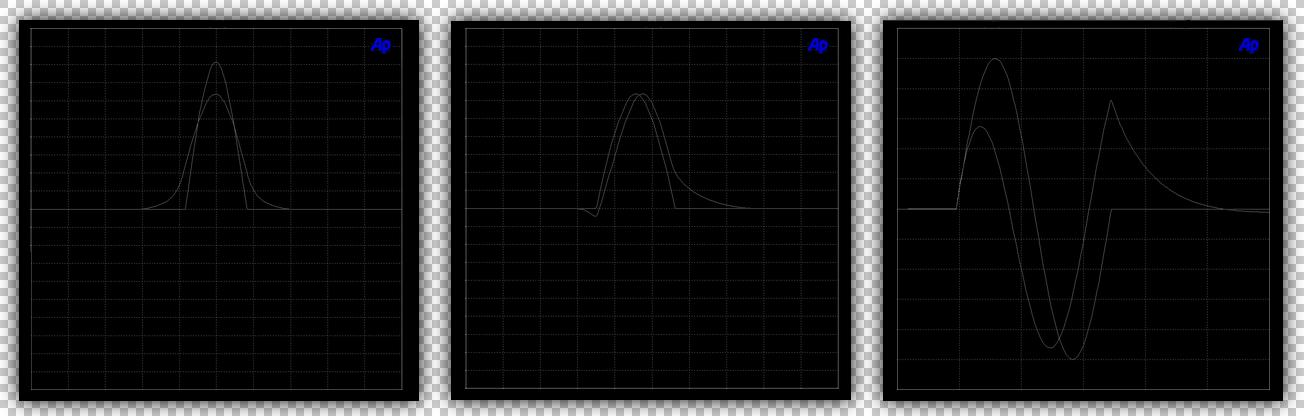
Above, the locked figures depict three instances of the same fundamental frequency. Each is superimposed with approximately equal quantities of third-order harmonic distortion. The level of distortion is higher than we find in production amplifiers and is used for illustrative purposes only. The first image contains a large input signal, a smaller third-octave harmonic that is in-phase, and is the more common type of third-order distortion present in amplifier designs. Also shown in the first picture is the cumulative effects of flattening upon the larger input signal. The positive magnitude (upward swing in the images above) combines with the smaller harmonic to form a steep rising and falling waveform profile upon the tone, now with a newly-reduced peak value. In other words, the crests are flattened by the harmonic. This also occurs in the negative downward swing.
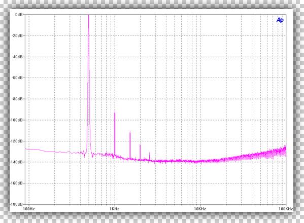
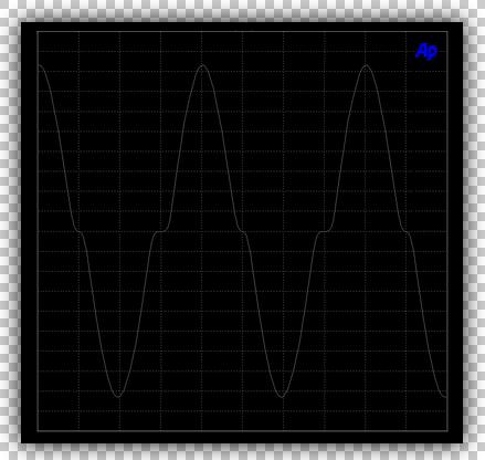
The second Figure to the right serves to represent how an out of phase third ordered harmonic can bring the primary tone to resemble a triangular waveform whilst it increases the peak value. In other words, changing the phase causes it to take an opposite shape. In Figure three, we see something rarely viewed or mentioned: a third-ordered harmonic who’s phase is independent from the primary stimulus, and for this scenario it resides at 80 degrees. Taking a long look above at these waveforms above and notice how much they change. While they are completely different from one another, each one appears identical in traditional Fast Fourier Transform analysis (F.F.T), thus exposing the first limitation of the common method of measurement, which I brought to light some years ago.
Third-order harmonic distortion is somewhat unique, because it is an order that can both decompose and accentuate the periodic function of a waveform with a mere change in phase. Thus, it creates a new hyperbolic or parabolic profile from the apparent difference of the two waveforms. Several year ago we found that, within a centric scenario where a third-order harmonic begins as an event with the same point and yet is out of phase with a fundamental tone, the hyperbolic effects did not act to flatten the crests of the signal. The results closely resembled that of second order harmonic. Later, several suborder classifications were issued to tangential third-ordered harmonic distortions, alone.
Building on this, it had been possible to create a number of amplifiers with equal magnitudes of third-ordered harmonics that measure the same in F.F.T testing, but which sound different from one another. This could be accomplished by altering the sequence of sine and cosine phase relationships between the fundamental signal to be amplified, and that of the source of the new harmonic multiple.
Higher order harmonic distortions can be even or odd-ordered. Where they bare no immediate correlation with the intent of primary signals, they are generally considered undesirable in the scope of audio reproduction. These tend to be quite low in amplitude within solid state designs. Yet, they can be pronounced in hollow state circuitry, in some cases descending only thirty-five decibels by the tenth order. In other words, they can be audible. Such is not to state any purported superiority of one above the other, but rather to clarify the nature of their behavior.
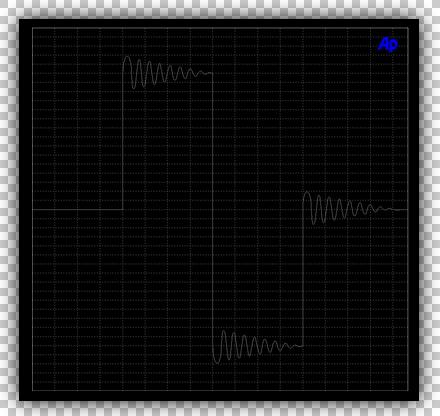
What is important about higher order Harmonic Distortion, is that when it has been permitted to reach high magnitudes the original sinusoidal waveform is gradually converted to a near-square wave profile. An actual square waveform will never occur normal audio playback unless the amp clips, but the affects are still important. It is rare for higher harmonics to occur alone, and those effects can be compounded to flatten the crest of an otherwise smooth and round sine signal. Adding to this, varying the magnitude of each order can produce waveforms that are slightly saw tooth or triangular in shape, as previously shown. Some types of distortion remains within a specific order and yet modulate in amplitude at the primary frequency, as depicted in the figure above. These stochastic behaviors appear ambiguous within the scope of most conventional F.F.T tests performed by conventional distortion analyzers. However, as can be seen here and possibly for the first time in the public domain, they are not one and the same, and they require that the tester realizes this.
In closing on this section, the fate of the life as we know it hangs in the balance of three things we have learned: Red is the highest maintenance color for a car, no matter how large that backyard deck is it’s still too small, and finally, if all the energy in a sinusoidal signal is contained at the fundamental frequency, then that signal is a perfect sine wave. However, if the signal is not a perfect sine wave, as it never is, then some energy must be contained in the distortion. In this way, energy is neither created nor destroyed, but remains a constant, and existing distortions can be accounted for. However, this does not imply that all distortions are simple harmonic multiples or can be described through this measurement alone.
Crossover Distortion
Another source of harmonic distortion is called crossover distortion. To fully understand the source, it is imperative that three amplifier classifications briefly be disambiguated for clarity. There are several alphabetical classifications for the operation of amplifiers, and they relate to the requirements and methods of biasing the active amplifying devices. Biasing the active devices moves them further away from their initial turn-on region and higher along their transconductance curves into their linear mode of operation. For audio reproduction, the bulk of amplifiers will be of the transimpedance operation common emitter and common cathode varieties.
Classification A amplifiers can make use of a single device, or multiples thereof in parallel, to conduct the entire 360 degrees of an audio waveform. They can also be built using even-numbered complimentary pairs of devices. In either of these cases, they are biased at the center point of their load line to a level that is half their intended maximum signal swing, known as the Q-point. This is done to permit symmetrical forward and reverse current signal reproduction.
Classification B amplifiers essentially always use even-numbered quantities of complimentary devices, with one reproducing the positive half and the other reproducing the negative half of the waveform. When one is reproducing half the waveform, the other is completely turned off and ceases to conduct. This type of amplifier is not biased, and typically is not intended for audio reproduction.
Class AB amplifiers employ even-numbered devices like Classification B types. However, AB designs bias the devices along the load line at a position that is above the “crossover region” where each device meets at 0, 180, 360 degrees, but the bias remains below the center of the load line. This constant-powered state causes each half of the complimentary pair to conduct for less than 360 degrees, but more than 180 degrees (half the full cycle), working to reduce and even eliminate switching transients. These amplifiers do not have to be biased near half their intended maximum signal swing, since the bias merge point between both devices forms this point. Even so, some Class AB amplifiers can be biased high enough to operated in true Class A.
While it may not be clear yet, Crossover Distortion can only occur when waveforms and signals are reproduced at current levels greater than the quiescent bias of an amplifier that use complimentary devices. When decomposed to its lowest common denominator, it can only exist where there is a transition, or “crossover” between two active amplifying devices, such as in Classification B and AB amplifiers. Crossover Distortion is quantified as a stationary harmonic distortion component that remains at a constant level and frequency, regardless of the input level and signal frequencies. The constant nature of this harmonic contribution means that lower level audio signals could be distorted more than larger ones, as a function of proportions. Put into perspective, the first one-hundredth of a Watt may be very distorted, while the one-thousandth Watt is exemplary. However, Crossover Distortion cannot exist in the power ranges below or equal to the quiescent bias value.
The lower voltage regions of some older devices exhibited varying degrees non-linearity. As such, should the bias voltage and current be too low in use, then, as the signal crossed the zero voltage potential points of 0, 180, and 360 degrees, crossover distortion could be introduced onto the signal. This became known as the solid-state sound of that time, although it was just as prominent in hollow-state designs that were biased equally. Devices dating from the nineteen seventies would have required exponentially higher quiescent values and still would never have achieved the unprecedented linearity available just one decade later. Very few audio companies provided harmonic distortion results at very low power levels, and this concealed the sheer magnitude of crossover distortion that was present. One company that would be the exception and deserving of recognition for their efforts, would be Yamaha Corporation, Japan. Working with Toshiba Semiconductors, Yamaha’s engineers literally wrote the books on measuring distortion and how to minimize their effects at low, high, and all levels in between.
Today, semiconductors and active devices have benefited from decades of electrochemical and physics research. It is because of the hard work put into the theoretical and physical, that crossover distortion among classification AB amplifiers is now largely a non-issue when properly accounted for. For many modern semiconductors, this linear region of transconductance is achieved with relatively small voltages and currents, and biasing eliminates the Crossover Distortion completely. As such, competently engineered Class AB amplifiers are capable of truly superlative performance, while those that have not, are not.
Most amplifiers employ potentiometers to allow adjustment of the bias points of amplifier’s voltage pre-driver and output stages. These center-tapped resistive controls allow the user to locate the practical balance between distortion and waste energy, but care must be taken that the quiescent current is neither too low, nor too high. There is a wide range where the bias level can reside with safety, but too low will allow the devices to turn off, imposing a variety of sharp transients on its output. Should the bias be too high, it could result in the premature failure of the devices being biased, or increase the induction noise from the associated power supply. Some designs feature automatic biasing that increases in steps with the output level. A very limited number of premier technology designs can even dynamically alter the bias in accordance with signal demand.
Intermodulation Distortion
Intermodulation Distortion is another non-linear behavior that can be found within electronics and stages of amplification. Abbreviated as I.M.D, this distortion is characterized by the appearance of an output waveform that is carrying bands of secondary emission frequencies, all equal to the sums and differences of integral multiples of two or more frequencies comprising the original input signal. As complex as this may sound, once one has a firm grasp on the origins and nature of the distortion they realize it is not so confusing. The primary difference between I.M.D versus harmonic distortion is that two or more different frequencies must be actively present to produce Intermodulation Distortion. This is different than the nature of harmonic distortion, which needs but one frequency to be present in order to form. Adding to this, Intermodulation Distortion products may not always be harmonically related to the original frequencies.
When a device under test is subjected to congruent signals – that is to imply that there are more than one signal at the same time – non-linearities inherent in that device will produce additional signal content at frequencies other than those present on the input. We have previously covered how an amplifier can produce even and odd-orded harmonic distortions, each being an integral multiple of the fundamental signal. In addition those, the Intermodulation Distortion will manifests as second-order and third-order emissions at every combination of first-order and second-order products, which are unrelated to the original signal. Adding to the harmonics, widely new spread second-order sub harmonic distortion products may occur below the primary signals.
The standard measure for this phenomenon is based on two-tone stimulus, best represented by an F.F.T graph. The Society of Motion Picture Television Engineers (SMPTE), DIN, and CCIF set the accepted industry standards for these tests, with the two primary classifications being I.M.D 2 and I.M.D 3 for the second and third orders of Intermodulation, respectively. The nature of this type of distortion is somewhat complex at first take, but it is quite easily and reliably modeled through convolution theorems.
Two of the most challenging distortion products in I.M.D tests are the additional signal content formed due to third-order distortion occurring directly adjacent to the two input tones. Regarding modulated signals, that is to say in two or more mixed signals with one or more following a pattern of varying amplitude, the third-order distortion creates additional frequency content in bands adjacent to the modulated signal, some subject to periodic summation. This distortion is known as Spectral Regrowth, and on an F.F.T graph it may be visually identified as a fattening and widening of noise spectra surrounding the primary tones.
There are a variety of means by which to measure this distortion, including interception for second order products caused by components that behave according the to Square Law. Another commonly used method is third-order interception, which is employed for artifacts introduced by components that behave in accordance with the Cube Law. Such is where the argument for higher priced and better engineered precision test equipment gains considerable ground, as lossy audio interfaces and low-cost analyzers will obscure the results among that of their own distortion artifacts.
Passive Intermodulation Distortion
We have established that intermodulation occurs as a result of an active non-linear system which is consecutively reproducing two tones. However, Passive Intermodulation Distortion, or P.I.M, as it is abbreviated, occurs in un-powered devices as the result of the two or more power tones mixing in the presence of physical device non-linearities. Examples of such environments that provide a situation for injection of P.I.M include the junctions of dissimilar metals like metal-oxide junctions, rusty screws, even loose connectors and solder joints. Another example pertains to radio frequency controlled aircraft, where should two metal surfaces physically vibrate against each other they can broadcast pulse-width modulated signals captured by the parts and then re-distributed. Passive Intermodulation Distortion may carry enough additional noise energy to swamp lower frequency two-way transceivers. It is also pertinent to audio equipment.
The higher the signal amplitude, the more pronounced the effect of the non-linearities and the more prominent quantity of intermodulation that occurs. Depending on the two fundamental waveform tones present, their intermodulation harmonics may add and multiply to completely obscure the target frequency. This holds great relevance, as even though upon initial inspection a system could appear to be linear and unable to generate intermodulation. Hysteresis in ferromagnetic materials can generate passive intermodulation products when such materials are exposes to reversing magnetic fields, and thus is primarily the reason why gold plating over zinc solder mask is omitted in some designs. Passive intermodulation can also be generated in components with manufacturing and workmanship defects, again, such as insufficiently terminated and cracked solder joints, or poorly made mechanical contacts. Passive intermodulation cannot exist in ordinary designs in the absence of amplitude modulation distortion. In some instances, the active componentry is much quieter than the passive components being used in conjunction with them.
Phase Response
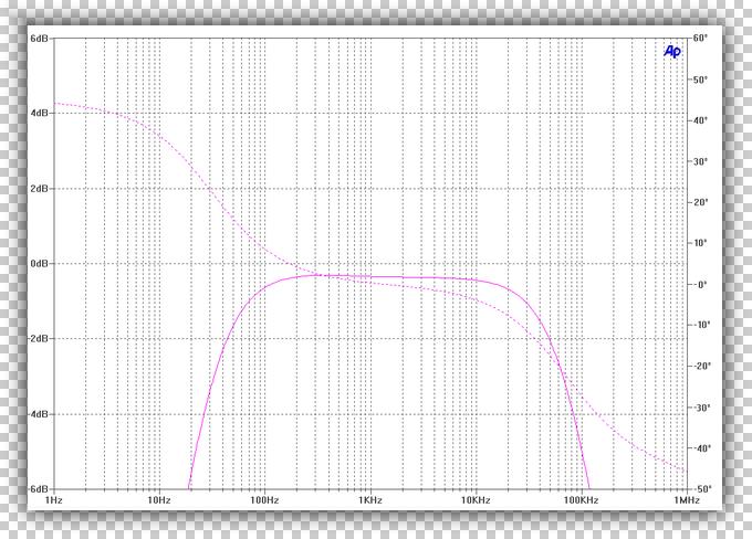
Phase Response is a means of representing the amount of change in phase that a device adds to frequencies as they are reproduced. Phase shift is expressed in degrees, and is used to describe the advancement or delay of phase in relation to the input signal waveform. A theoretically perfect amplifier with a perfect phase response would introduce an change in phase at all frequencies reproduced, thus having a net phase of zero. The unfortunate news is that nothing in our world is perfect, including amplifiers. The uplifting news is that we can design audio amplifiers with a Phase Response of single-digit values or better, where the effects are of little importance.
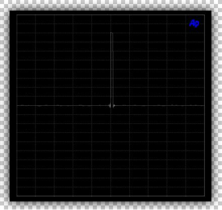
Phase shift and phase delay are often one and the same thing. Phase shift typically occurs at frequency extremes, and phase shift will typically be minimal throughout the mid-band frequency region. Most production home audio amplifiers have less than -10 degrees near 20kHz. This corresponds to a 1.4 microseconds (µS) delay period at that frequency relative to other lower frequencies. This amount of shift is mostly insignificant, even among the most demanding live audio applications.
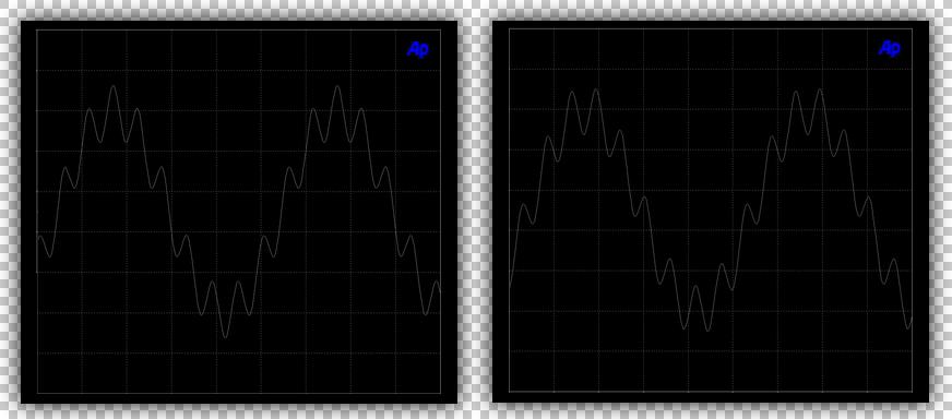
In the Figure above, two scope images have been captured. In the second image above, the effect of excessive phase shift may be readily depicted by the difference in the relation of the higher frequencies on a carrier. When this occurs during music playback, the timing cues fall out of sync and quality of timbres are changed.
It is much more common to see larger phase shifts in the lower frequency regions, as a function of the direct current blocking and high-pass attenuation circuitry. The phase becomes more problematic as frequency is decreased because, as signals descend the frequency scale within a decade, the shift in frequency timing becomes more audible to the listener. Amplifiers that display high quantities of phase shift also introduce large delays to frequency components that occur in the correspondingly higher phase regions. If we were to investigate the relationship between slightly higher harmonics and a carrier frequency of 20 Hertz with 10 degrees phase shift, the bass and harmonics fall out of timing by 1.4 milliseconds (mS) – much longer than the equivalent shift at 20kHz (1.4 microseconds [µS]) .
In the Figure above, there are two low frequency waveforms without any harmonics. These waveforms should be the same but, they are quite different. The grey waveform is the input signal, and the output signal is shown in blue. For this arbitrary circuit, the high degree of phase shift that is present leads to the gradual build-up in signal strength and additional distortion as the signal ceases. This is an example of an audio device that will demonstrate poor bass impact, regardless of how large its power supply is, and despite the fact that is measures mostly-flat with continuous sine signals.
In audio, a millisecond is a long time wherein many events can occur. One can pull a variety of audio components from the shelf to find phase deviations larger than this. An example includes hollow state thermionic valve amplifiers that may have as much as 60 degrees phase shift at 20Hz, which is associated with their passive cathode biasing and direct current coupling capacitor value choices. At 60 degrees and with 20Hz signal, the result is a8.35 millisecond deviation which leads to the notable attenuation and alterations to the waveforms. It invariably contributes to the destructive breakdown of the original harmonic and organic beat structures found in natural sounds.
Phase Response and impulse response go hand in hand, although they have been separated in this article to disambiguate their interpretations. Phase Response is also different than transient latency and physical delay, which will have their own section. Because Phase Response occurs in the frequency domain, it is classified as a linear distortion mechanism.
Absolute Phase
Absolute Phase, which is often confused with the term polarity, applies to the apparent direction of signal swing for a given period. In other words, an electronic component with Absolute Phase integrity would maintain the signal’s phase relationship. In this way, positive swings in equal positive swings out, in that order. In terms of a practical audio system, it can be more readily depicted through visual demonstration of low frequencies being reproduced by large loudspeaker with an adjacent oscilloscope, or other device to show the signal coming in from the source. For example, when a signal is on a positive swing, a system with Absolute Phase will cause a low frequency driver to accelerate in a forward fashion. A system with opposite phase will cause a loudspeaker driver to move in the opposite direction, even though the original source signal was on a positive swing. Phase measurements are taken at the device’s outputs and are then compared directly with that of the input.
“Phase is not only inherent in an audio system, but also applies to the recorded media, or other sources of reference. This is called Relative Phase.”
In consumer home audio, some electronic audio components have been designed with inverted phase outputs. This was a common case among hollow-state preamps and simplified solid-state methods of gain control, before the inception of lower-noise devices. In more recent times, designers have opted to preclude phase inversion, and in essence, nothing was lot in gaining Absolute Phase. The reasoning behind the ideology is sound that if the phase must be revered, it should not affect every source. Many people are unaware that their system may reverse the phase of the input signal. However…
Phase is not only inherent in an audio system, but also applies to the recorded media, or other sources of reference. This is called Relative Phase, and although not deserving of its own section it does warrant some mention. Not all recordings are phase correct, and this is particularly true of some vinyl pressings. As a result, some manufacturers include a phase inversion switch on their phonograph stages to allow the listener to decide what sounds best to them. While extensive studies and recording professionals suggest that the auditory system is insensitive to an asymmetric sinusoidal signal, it is also suggested by sources that this may be best left to the end user to determine.
Latency
Latency is a condition where the output signal that has been reproduced by a device is delayed so that it is no longer instant when compared with the input signal. Some analog circuits are constructed in such manner that there may be latency, thus we observe a distinct difference in alignment between those two signals. This becomes important when the audio, or other signal, has to be referenced against another live event, such as video. Digital audio processors introduce the greatest timing error, as any digital interface operates upon the principle of data sampling. The time that it takes to collect and process this data determines the apparent Latency. Latency is usually uniform across all frequencies pertinent to audio reproduction, and the gross difference occurs between events as a perceived lag in time.
Oscillation, Stability, and Phase Margin
The Stability of an amplifying stage indicates its inherent immunity to a condition known as Oscillation. Oscillation is the sustaining of a signal at the output after the input stimulus has ceased. Oscillation can be self-induced or result from an external factor, such as when a reactive load is placed at the output of an amplification stage. It is important that the chances of oscillation be mitigated, otherwise, the cause of the oscillation may build the signal magnitude to such point that it overdrives the amplifying device, possibly damaging it and the load.
Every device, be it semiconductor or thermionic valve, has an upper frequency limit where its phase reverses 180 degrees. This is a naturally occurring part of electronic and mechanical bodies. The first-order corner frequency for an active amplifying device may reside near one-Megahertz (MHz, million cycles per second), while that among logic devices may reside in the low Gigahertz {GHz, billion cycles per second). This pole causes high frequencies above it to attenuate at six decibels per octave, corresponding to 20 decibels per decade. It will continue to attenuate at this rate until it merges with another pole. This is a single time constant, and the device will continue to attenuate at this rate until it merges with another pole.
An amplifier with a single time constant and zero phase shift at unity gain (unity gain refers to no reduction or increase as the signal passes through the device, gain equaling 1) is always stable, but many active devices have at least two primary poles at unity gain. The second pole attenuates at a rate of twelve decibels per octave and 40 decibels per decade, twice as high as a single time constant. If the active device is among those who’s frequency response naturally drop below unity gain before this second pole is encountered, it will be unconditionally stable at any gain level. If the 2nd pole is encountered above unity gain a gain of 1, special attention will be required for some implementations. In a few moments we’ll take a brief look at how that gain is determined.
The stability of an amplifier is represented by its Phase Margin (P.M.) in degrees, where the stated value implies how great the normal-state phase is from the 180 degree point. If the amplifier’s phase margin reaches 180 degrees by a shift that is superimposed back onto the input through parasitic paths or design errors, this condition will permit oscillation. Phase Margin is also indicated by what is called the k-factor. A K-factor of 1.0 is a boundary condition for unconditional Stability, and a device that has a k-factor of less than 1.0 is only conditionally stable. An amplifier with a k-factor of 1.0 will not oscillate, regardless of the signal being applied, the source impedance, or the load phase angle.
A device operating without negative feedback is known as open loop. This condition offers the highest possible resistance between the input and output of a device, and little to no interaction. It results in limited high frequency response, high levels of distortion, and gain which is often to high to be useable in audio applications. Feedback can introduce some levity upon the situation to greatly improve several parameters of the device, and it works by trading gain for higher linearity and lower distortion.
When a conductive or resistive path is placed between the input and output, it is known as a closed loop. For most audio applications, a localized negative feedback loop will be the most common type of feedback, featuring a closed loop with a resistive or conductive medium to set the desired gain. As the resistance is decreased, more feedback is applied and the gain is reduced. The bandwidth increases and the distortion decreases.
Feedback is an often confused concept, as it does have a learning curve. Many believe that it is the act of taking the output signal of a device and sending back to the input. This is incorrect, as feedback is a method of taking the output Voltage, or portion thereof, and presenting it back at a devices input. While these two concepts appear identical, they are not exactly the same. This distinction becomes most important as one advances.
With enough feedback, the amplifying device may reach the device’s 180 phase shift point. To allow the device to safely be used high feedback, a small value compensation capacitor, called a Miller capacitor, may be placed in parallel to the resistive feedback loop. This is used to cause the circuit to act as a phase advancer, and attenuates the high frequency gain. In doing so, it helps to keep gain at ultrasonic frequencies from reaching critical symmetry, where the feedback would otherwise become positive and produce some level of oscillation and distortion.
We know the net result of feedback is a flatter transfer gain over the designated bandwidth, much lower distortion and Miller capacitance helps prevent instability. Attenuating high frequencies or moving the poles upwards in frequency allows more feedback to be applied, and thus, improved linearity. However, there is an important balance that must be weighed in to ensure that high frequency integrity is not compromised. There is a point where a given amplifying device performs its best, and where too much feedback for specific devices will require excessive compensation, compromising the slew rates.
On your audio journey, you may have heard mention of something called Zero-Feedback. Zero-Feedback is often used in the audio industry to claim an audio amplifier as being bereft of any feedback. It is both a misnomer and erroneous descriptive mechanism for how the amplifier is designed and operates. What perhaps should be stated in its place, is that the design uses near-zero decibels of X-type feedback or zero global feedback, which ever is applicable to the design. This is because there are clear feedback paths on the schematics. Several others in the industry have also echoed that each one claimed to be bereft of feedback had been quite the opposite – those designs simply traded global feedback for localized loops. Others make use of a closed loop, but where the high resistance value brings the gain close to open loop, they label it as zero-feedback as though that were constituent of zero-feedback circuit.
The single notable exceptions are a couple transconductance designs that have gone and resurfaced over the years. They utilized autoformers for voltage gain, feeding a pair of Jfets or Mosfets. These still use passive or active degradation, which in itself is a type of feedback. In these designs, the absence of negative feedback comes at the expense of distortion, poor output impedance, and a very limited bandwidth. The scientific engineering fact of the matter is that any amplifier that uses a non-zero resistance, or impedance on the cathode, emitter, or source drain, is by definition using feedback. For example, single-ended Classification A amplifiers mandate the use of a passive and sometimes active cathode or emitter resistance (sometimes in conjunction with a capacitive reactance to entice improved low-frequency extension) to place the Q-point approximately half way along the load line. This constitutes degenerative feedback. Should there be no resistance or impedance, the amplifier no longer reproduces audio waveforms.
There are also a wide spanning variety of different feedback topologies. Not all feedback is the same, nor serves an identical purpose, and all must be executed intelligently. Among the varieties there is positive feedback, negative feedback, thermal feedback, voltage feedback, current feedback, feedforward, global feedback, ERCO, and the list goes on. Every production amplifier uses controlled feedback to improve its linearity and stability. It also greatly reduces the output impedance of the circuit, making it more better suited to driving changing loads. High Current is actually a misnomer for high feedback.
Another important area of stability in amplifier design brings us to the output portion and the load that it is connected to. The amplifier interacts with a non-linear speaker load having a reactive impedance which changes with frequency. Given the situation of impedance, phase Theta is the time difference between the peak voltage and peak current. In other words, impedance is the phase difference between the voltage and current. The impedance of a speaker cannot be both inductive and capacitive at the exact same frequency. Instead, it will vary as frequency is altered. At resonance, a driver is resistive; below this point it is inductive, above this point it will be capacitive, and eventually series inductive once again.
The more reactive that a load is, the greater the margin of misalignment between these two prime constituents. An amplifier will have a degree of sensitivity to the phase of the load it is driving, and as the phase approaches full reversal, it will begin to ring. In addition to thermal stress, a high degree of phase shift is the the most challenging load faced by an audio amplifier. It can result in heavy waveform deformations and even lead to an amplifier’s failure. Despite marketing commentaries to the contrary, irregardless of how powerful an amplifier is into any impedance load, its stability remains independent of that power. The only connection is that high feedback promotes a low output impedance, while the stability of that feedback is still separate.
One final part to mention, is that the power amplifier is connect to the loudspeakers via a long cable. Therefore, any parasitic radio frequency interference that may be picked up by the speaker cable may find it’s way back onto the amplifier. External causes of instability originate from the interception of a frequency corresponding to an existing pole, or symmetrical phased electromotive forces. An amplifier that does not naturally attenuate radio frequency interference on its own requires a low pass filter, or the isolation of critical components to prevent radio frequency interception. Radio noise commonly finds its way into high speed amplifiers, either on the input leads or on the loudspeaker cabling. From there, it progresses onto the power rails and may present a loop. Several forms of isolation, such as shunting with capacitance, can prevent the introduction of transients and other undesirable signals from being intercepted by a gain stage. In larger power amplifiers, the requirements of a small value output choke is often mandatory, whereas in smaller power amplifiers or voltage gain stages, it may be omitted in some designs without repercussions.
In closing, the phase margin for stability is rarely provided among consumer audio products. It is sometimes believed that amplifiers oscillate when they clip, but this is not the case.
Frequency Response Function
Often abbreviated as F.R, Frequency Response is a quantitative measure of how precisely an electronic device under test maintains a constant output signal amplitude over a bandwidth, while the input reference signal remains unchanged. Among scientific bodies, Frequency Response Function is also often referred to by the name Transfer Function. Deviations from a flat frequency response occur in the linear distortion domain, and gain flatness indicates the variations in the device’s static gain behavior over a stated frequency range.
When a recording is produced, it is assumed that a linear playback system will be utilized, so that it is capable of reproducing the same energy at all frequencies in accordance with our own auditory system. A flat frequency response is indicative of the overall quality and ability to respond to upper and lower harmonics of signals, all the way to the extremes of the audio spectrum. In order to reproduce music with a degree of faithfulness, it remains important than an audio system be bereft of any traits of accentuating, nor attenuating the frequency response in the audio range. However, there is nothing wrong with a listener preferring to tailor the response to their preference.
Because extreme stability is necessary for some types of sound applications, some manufacturers have made provisions for early filters to restrict the frequency response, or have allowed for relatively high distortion in return for increased amplifier stability. This is because electronics devices have a specified bandwidth in which they will offer their peak performance and safety, and it just happens that the human auditory spectrum extends over a region where that bridges both low and high frequency devices. However, the later half of the 1980’s saw the introduction of the next generation of semiconductors and those which not only replaced all the forebarers; but have remained the basis for essentially all modern devices used in audio, many of which are still in production.
What has changed since that time has been that newer iterations of obsolete devices have become more efficient and offer lower noise. Among a variety of parameters, they offer a lower input capacitance and higher safe operation points. As a result, they are more flexible in usage, can handle greater thermal and operational stress, and are easier to drive with less demand upon requisite componentry. Even so, it has been fully possible to obtain excellent frequency response for several several decades. The frequency response of an audio component will, however, be limited by the designer. All finished amplifiers that employ devices in a closed loop manner will feature a low-pass filter, be it passive or active. This is to improve the safety of the amplifiers, and to prevent them from self destruction, or acting as a radio frequency transceiver, ie: a radio receiver and broadcast transmitter.
Where any situation arises that an audio reproduction amplifier has no active means to suppress such signals, it would be increasingly dangerous to allow such a product to operate in a manner permitting a high frequency signal (that corresponds to upper poles) to make its way onto the input. Equally concerning, would be the introduction of a lower frequency (for example: 200kHz-1MHz) radio transmission upon the amplifier’s signal input interconnects, or internal traces, then being amplified out of phase and having that voltage signal on the output superimposed back onto the input. The lower frequency limits of an audio component may also be limited to attenuate power-robbing subsonic frequencies, or to mitigate direct current transients from damaging the loudspeaker system. A key designer with experience in signal processing will be able keep the frequency response flat, typically within a couple decibels from 20Hz to 20kHz and beyond.
In most cases, upper frequency extension to 100kHz is common and this is more than adequate for music and theatrical audio reproduction. This frequency is several octaves above and beyond the limits of the perceivable audio spectrum, due to the mass of the tympanic membrane, the hammer and anvil, their shape, and the genetically designated operation of the cochlea. Also, this is far beyond the scope of analog and digital audio recordings that are available, as per the mechanical, electrical, and Nyquist theorem; the maximum possible frequency is one half a digital sampling rate, and aliasing distortion becomes prominent prior to this being realized, thus necessitating integral filters.
The real Frequency Response will vary from the asymptotic response as a direct result of the small signal capacitor’s (where applicable) inherent high equivalent series resistance. The compact cost-saving surface mount capacitors in modern gear may have a stated capacitance of as much as 10uF, which depending on the following circuit impedance, may be more than sufficient. What is important to note, is that under certain thermal conditions the effective value decreases to as much as one-tenth that original measured value. While it is difficult to validate the use of capacitors that cost thousands of dollars, there is an argument for poly film types, and that they are reliable, display lower distortion and have better consistency with thermal rise. This is a condition in some applications which may not be consistent, or monotonic. The flip side of this situation is that larger value capacitors require a greater quantity of energy to sustain the charge-discharge cycles of an alternating current signal, exactly like we find in audio, for example.
With proper filter points chosen and phase distortion greatly reduced, a new problem presents itself. We can ascertain the output, or a leading stage is AC coupled with a capacitor by the presence of residual DC after the signal has stopped. One would ask themselves, “How could a direct current make it through a DC blocking capacitor?” The short answer is that whilst the capacitor is charging it has to pass current. During that charging cycle, the zero-offset point is disrupted. A concern unique to AC coupled monolithic systems stems from these apparent duty cycles wherein the crucial center reference point should have a potential of zero Volts; an AC coupled stage can introduce headroom issues as low frequency bandwidth is increased, since half the waveform will shift from zero offset and may exceed the clipping threshold with dynamic signals at these low frequencies.
A skilled engineer can decrypt a great deal of pertinent information regarding the design of a component, based on this criteria set. These include nodes and modes, phase margin, stability and other concerns, and they can also be derived from the slope types. Certain behaviors are indicative of the topology, and they can also serve as indicators of other aspects of reproduction fidelity, too. A response that begins to heel within the audio bandwidth is a sign that there will be phase shift associated with those frequencies, where a non-linear slope that is shaped or steeper than six decibels per octave would be descriptive of a multi-pole filter, usually achieved via successive staging.
Power Bandwidth
A device’s power bandwidth relates to the frequency range that it covers at a stated power level, usually stated in Watts or Volts depending on the application. A frequency response measurement is captured at the relatively low power output of about one Watt, known as small-signal bandwidth. The Power Bandwidth of a product contrasts to the small-signal analysis, and it is measured at the half-power or full power capacity before the onset of clipping. The Power Bandwidth measurement provides a reliable and accurate means by which to quantify an audio device’s ability to produce high levels of output over a wide frequency range. The limits of the power bandwidth are defined by the points where the product can only produce half the power that it was capable of at one-thousand Hertz, ie -3 decibels. In a well conceived design, this will reside far outside the audible regions.
“While some may associate that sound with under-built power supplies, it is rarely the induced by such. It was often the result of employing early low frequency devices while reducing the number of successive stages, and operating those devices at too-high gain product levels.”
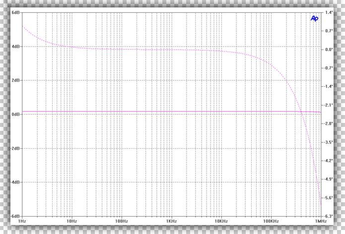
If you have ever encountered a vast reduction in the bass or treble levels of a system as volume was increased, you may have experienced the audible artifacts stemming from the limits of the Power Bandwidth. Sometimes abbreviated P.B. or G.P.B for Gain Power Bandwidth, it relates to behaviors wherein as the device’s output level or gain is increased, its frequency response narrows conversely. This is because the frequency response of a conventional transimpedance amplifier is inversely proportional to the gain. As the output level or gain is increased the bandwidth is subject to reduction, and this can be depicted with what is called a Bode plot.

The above Bode plot illustrates the open and closed loop gain and Power Bandwidth for three different feedback levels. The higher line that intercepts the Bode rate of rolloff depicts the least quantity of applied feedback (40dB) offering eighty decibels of gain, but also narrow full power bandwidth (Fp) of 1kHz. The next line down shows the 60 decibels of feedback, providing 60 decibels of gain an Fp bandwidth of 10kHz. Finally, the lowest intercepting line depicts eighty decibels of feedback and forty decibels of gain, offering a Fp bandwidth of 100kHz. As more feedback is applied, gain is traded for improved linearity and frequency extension. However, if the bandwidth becomes so wide as to intercept the device’s upper resonance pole above a unity gain of zero decibels, and the rate of attenuation exceeds twelve decibels per octave, compensation will be required for stability.
In the earlier days of solid state, devices displayed a narrower Gain Power Bandwidth. What that meant, was that if the device was used without feedback, or was operated at high levels with low feedback, it would be entering the power region where its associated frequency response was the narrowest. As a result, this could cause the crescendos and dynamic swings to fall short of their proper frequency spectrum and even distort, resulting in the sound becoming compressed and constrained. While some may associate that sound with under-built power supplies, it was rarely the induced by such. It was often the result of employing early low frequency devices while reducing the number of successive stages, and operating those devices at too-high gain product levels. In other words, it was not the collective fault of the power supplies. The later updated wide-band high gain versions in the 1980’s made Gain Bandwidth Product issues in audio equipment design an obsolete topic, but caused some new troubles for a number of audio companies that were not prepared to take full advantage of the high bandwidth. That was readily evident in their written disclosures, if not overtly apparent in their design choices.
The power bandwidth of a properly engineered amplifier, or other gain stage is quite linear from 20Hz to 20kHz from a fraction of a Watt to full power. In some cases, it approaches one-Megahertz before a low-pass compensation filter is installed in the feedback loop, or elsewhere. The response should remain constant at audio frequencies, regardless of power output. Taking the example of an amplifier for instance, wide power bandwidth means that the device can reproduce high level upper harmonics within a signal at any power level as easily as it can reproduce mid-range fundamentals. The end result of a properly designed amplifier with a good Power bandwidth it that the listener gets full power-performance from the product over the entire audio frequency spectrum. It is especially important when the amplifier is called upon to reproduce musical material with high energy over a wide frequency range, where perceived sound quality on dynamic passages may otherwise become compromised.
Gain Factor and Small Signal Gain Linearity
Gain is the relationship that exists between the relative signal magnitude found on the output of a device compared to that which exists on its input in the same instant. Audio equipment, including phonograph amplifiers, preamplifiers, and power amplifiers, each have a quantity of gain that can be represented as the ratio of voltage signal multiplication as waveforms are passes through the device. This multiplication is the increase in level and is known as amplification. Amplification can also take place in the current domain while at vanishingly low voltage potentials, however, very few audio components are designed to operate in this manner. The final value of signal multiplication may be given as a Gain Factor ratio that compares the output to the input, or, simply represented as the amplitude in decibels. The latter is much more useful for the general public, as it relates to something that everyone can relate to, respectively.
In this modern age of home audio reproduction circuitry, Gain Factor is usually a fixed value. Power amplifiers often provide twenty-five to thirty decibels of gain, enough to preclude any need for a preliminary stage of amplification and allow them to be driven to their maximum output power. Control over the output level of amplification is adjusted by a potential divider network that has been integrated into an early stage prior the power stage, and as mentioned, this early stage may not offer any gain. Sources, such as compact disc players and phono amplifiers normally operate at the one to two-Volt levels. These are typically greater than what is necessary to drive most power amplifiers into hard clipping. Lower level sources and quieter recordings may require more gain to achieve the desired playback levels, and these are the primary reason why the vast majority of discrete preamplifiers do offer active circuitry and gain.
Throughout the history of consumer audio design, there have been cases of products which operated under conditions that precluded them from being capable of providing linear dynamic reproduction. What these devices did was mute, or otherwise compress the apparent signal while remaining bereft of any signs of clipping. The two primary scenarios can be decomposed into the following: muting of small signals, and the compression of dynamic passages. The former instills a loss of information that comprised the finer and lower-level transients in a recording. The latter encompasses a situation wherein the peaks above an unspecified margin are reduced in amplitude. Building upon this second deviation from gain linearity, there may have been provisional instances of small signals being left unchanged and the proportions maintained perfectly, yet dynamic range reduced. This peculiar form of gain linearity distortion made smaller sonic traits appear louder, leading to the impression of great detail, while maintaining a very limited dynamic range.
There are two main types of amplification; current and voltage. Voltage signal amplification is the most common and remains the simplest. Current amplification is a means of signal transfer which largely diverts the problems of stray parallel conductor capacitance in long runs. Provided that the signal path can offer a consistently low resistance, there is little signal degradation. It works by feeding stages with a a current signal at resides near nil Volts. If one were to attempt to measure it with a multimeter, it likely would behave as though no signal was present on that line. In order for current flow to exist, there has to be a voltage. In the case of current amplification, it is simply such a small value that it escapes detection by typical low-sensitivity measurement gear, such as multimeters. This very small value of potential is not unlike that amongst digital logic circuitry and digital to analog converters, and maintains this current flow integrity through the use of low resistance circuit networks.
At some point, preferably closer to the final stage, the input signal must be converted into a voltage for it to be useful. This is really quite simple and only uses a single stage, such as an operational amplifier with feedback that serves as a transimpedance converter. The operational amplifier is the most common method of conversion due to its inherent precision. The line input to the stage is taken at the negative-designated input while the positive input is shorted to a ground plane. Any current flowing into the negative input will have to flow through the feedback resistor, which will develop a voltage across this resistor as per Ohm’s Law. Operational amplifiers are designed to prevent any differences from occurring between their positive and negative inputs, as they are effectively a V-to-I converter that cascades into an I-to-V output stage. The negative input will effectively act to mirror the positive input, which means the negative input is effectively grounded as well. If negative input and output are indirectly connected through a resistor, as with feedback, the output stage must compensate for the voltage drop across the resistor. Voila, thus converting the current into a proportional voltage signal for amplification.
This can also be accomplished with a vacuum tube, but it is important to maintain a high interstage or source impedance. Where most audio components strive for low source impedance values, a tube (such as a triode in an I-to-V stage) requires a high source impedance to enough permit freedom for the grid to move. Designing a high impedance source has never been a difficult task. Simply increasing the driver value of the cathode resistor in a grounded cathode triode amplifier will place the impedance very high.
“Not all of the various types of distortion exhibited by electronics can be demonstrated by sinusoidal test tones, nor under steady operating conditions, alone. It has been devised that during years of audio component engineering and research design, this has been one of many great lessons. An interesting portion of this casual article may be that of the dynamic classifications of distortion, as they demonstrate that static measurements do not always reflect the complete behavior of the dynamic modulus like we encounter in music reproduction.
In other words, the tests we see online and in brochures are those of steady-state sinusoidal tones, and they focus more upon the behaviors that are only seen as a signal continues onward. However, musical signals initiate, cease, or otherwise change. No two arrangements behave in an identical manner under all conditions.
All audio waveforms are comprised of carrier waves and additive and subtractive components, and therein the alteration of shape, proportion and frequency forms the final dynamic audio product. Those measurements serve to better reflect the way electronic products reiterate audio waveforms. In light of this, it is interesting that even in this day in age, some still assume that two to three static tests are descriptive of the device in its entirety. Furthering this paper, we will now enter the topics of more intricate forms of Dynamic Distortion. Whilst several of these distortions are most pertinent when applied in the context of physical mediums, each also holds credence in electronics engineering.”
Amplitude-Frequency and Phase-Frequency Distortion
Some types of distortion act differently, depending on whether the fundamental frequencies are continuous, limited to a single cycle, or even portion thereof. As such, distortion analysis based on test tones overlook a great deal of behavior exhibited by the device, leaving much of its performance and sound a mystery to the uninformed. None of the following are represented in a typical F.F.T through a tone test. The following is a small compilation of test results and the classification of each.
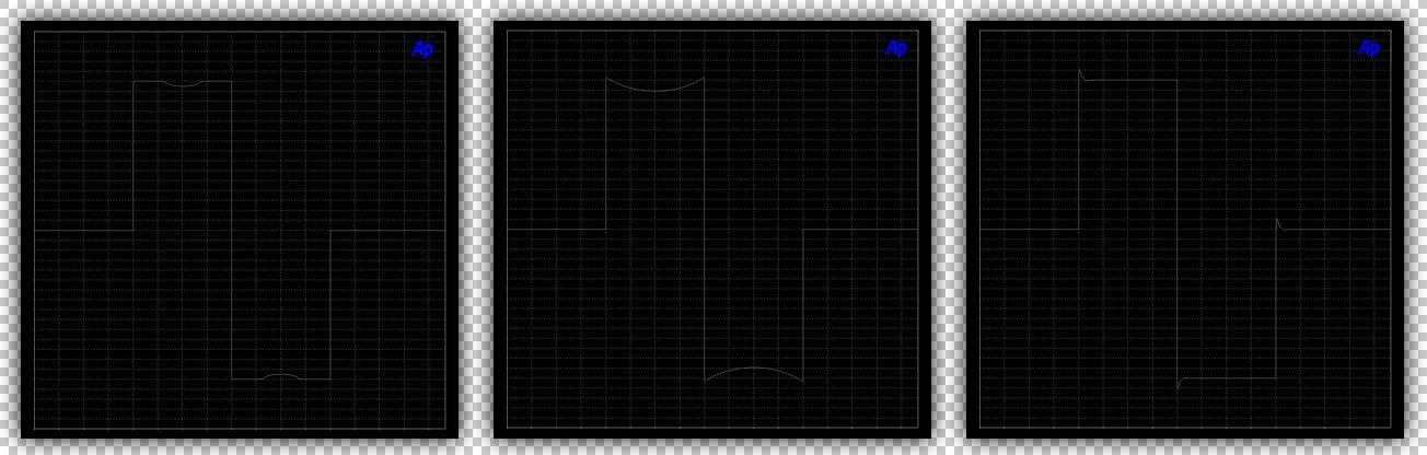
The Figure above displays Amplitude-Frequency Distortion, Phase-Frequency Distortion, and the cumulative results of phase shift upon a tone spanning several cycles. An example of Amplitude-Frequency Distortion is present in the first image. This type of distortion results from form of change that typically involves a half waveform, or an otherwise sinuous transient, who’s amplitude is inceased or decreased. Meanwhile, the timestamp is also altered to change the frequency. This is a complex distortion, and it completely changes the original transient content to such extent that it no longer resembles the original signal.
Much like Amplitude-Frequency Distortion, Phase-Frequency Distortion is a situation that arises when a circuit imparts a difference in apparent phase, resulting in a modification of the impulse’s time span. After arriving at the distant end of an audio circuit, the currents require time to build to their intended value. However, if conditions dictate that the time envelope needed is far too great, they may never reach their previous levels. This of course results in the attenuation and distortion of the signal’s initial & terminating pulses. It is possible to have a device or circuit that exhibits both the traits of Amplitude-Phase Distortion and Frequency-Phase Distortion sanctimoniously.
In the third Figure, we can see an example of what phase can do to a complete sinusoidal waveform. The initial point of 90 degrees fails to reach its intended peak magnitude, and where the out of phase signal ends without completing its full cycle, it ceases with an abrupt transient spike. While this can happen at any point over a device’s bandwidth, this type of behavior is most often present at low frequencies. Anywhere there is a low or high pass filter, there will be some phase shift.
In many commercial and DIY designs where undersized coupling values are chosen to lower build costs, or simply because they are deemed adequate, the above Figures display the results. Bypassing the small film signal capacitors with 10µF, 27µF, or even 100µF electrolytic types goes a long way to reduce this aspect of phase distortion. Have no fear of the electrolytic polluting the signal or otherwise mitigating the purpose of the smaller and higher quality primary film capacitor, because the equivalent series resistance and inductance of modern films is far lower than that of electrolytics. Thus, the electrolytic is more resistive, and thus only active where the film capacitor was otherwise ineffective – at low frequencies.
Amplitude Modulation Distortion
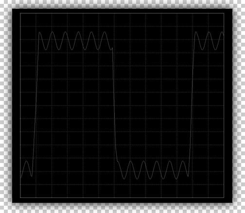
Amplitude Modulation is technique used in signal broadcasting and pulse width modulated means of amplification. There are three primary types of amplitude modulation distortion involve superimposing a carrier signal upon the fundamantal signal: This signal may maintain a constant dominant tone and vary in amplitude proportional to the fundamental signal; it may operate at a constant dominant magnitude and wave in frequency with the input signal; finally, it may track the input tone, following as a small signal anomaly.

The first Figure above demonstrates an example of Amplitude Modulation Distortion acting on a square-wave primary tone, as previously mentioned in the section pertaining to harmonic distortion. The second Figure demonstrates a third-order harmonic that modulates in amplitude at the same frequency as the fundamental sinusoidal waveform. Where audio is ever-changing, the effects will be more pronounced with some music and media than others. Adding this factor to a change in phase of different harmonics, the cumulative effect can be dynamic.
Any time that amplitude modulation is not part of the primary design goal, it should be treated as a parasitic effect and the source soon after located and the cause rectified. Amplitude modulation can apply to any order of harmonic distortion, where the harmonic contains an amplitude modulated sample of the fundamental frequency. In this case, the rise and fall of the waveform remains close to the original, but the crest is suppressed by the out of phase modulation.
Transient Response
Transient Response encompasses important aspects of audio reproduction and design. The term is broad, but implies the importance that a device under test be transient tested to help quantify its fidelity in recreating stochastic multi-state trajectory, in combination with other signals. There are a number of tests for Transient Response Distortions, encompassing large and small signal tests and multiple tone signals, and a variety of methods that demonstrate how the subject behaves under dynamic conditions. Transient analysis differs from other tests, because it employs specialized methods and a variety of stimulus which may not recur, whilst harmonic and intermodulation distortion capture techniques centralize upon steady-state ongoing sinusoidal waveforms.
The primary reason for Transient tests is that all sounds and musical signals have both a beginning point and end, sometimes abrupt. The criteria for these signals is constantly changing in terms of amplitude, frequency content, beats, modulation and the additive and destructive interference of such contributions. I other words, music and natural sounds contain distinct transient events which are both brief and quite asymmetric in shape. There are a number of different tests for transient response, and each is based on creating data when a device is requested to rise or drop from a potential of zero to a new set point of magnitude, possibly even maintain that level there for a period, then reverting back to zero potential. A competent and experienced engineer can gain great insight about the circuit topology, the mode of operation, the nature of filters and other important behavioral characteristics of a device. These can be determined based on comparison of the results with known performance criteria.
The secondary reason for testing Transient Response is spearheaded by the fact that many stages of signal processing and amplification behave slightly to vastly different in their ability to handle impulses, square and triangular waveforms. While very few soundtracks contain perfect square waveforms and the sound of such is of little concern, it is not so much the reproduction of a square wave that is always of interest the prudent designer. Instead, it is more often what exactly is added during the inception of those impulses or waveforms. Any additional tones or pulses that this stimulus may spark great interest and help the engineer to build a better sounding, safer device.
Impulse Response Function
Impulses are short duration transients, meaning that the events are a brief occurrence. There are a number of techniques for the analysis of impulses, and amplifiers are generally treated as discrete-time systems, rather than introduced to a continuous cycle of impulses. The electrical transient comes from a precision calibrated source, such as a laboratory function generator and comparator. The intent is to create a fast rising pulse that sharply squares off at its peak, then falls equally fast to zero potential. The value of this test is realized in the observation of how a device under test behaves immediately leading up to and following the impulse.
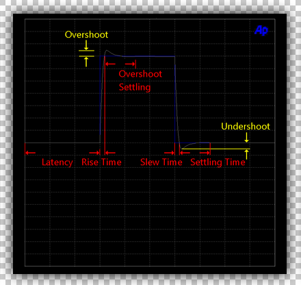
Impulse Response Functions, abbreviated as I.R.F, are common in dynamic power testing of amplifiers, but is also a good tool for identifying problems with small-signal reproduction which could lead to a perceived loss of sonic information. The Impulse Response Function of a device can be derived by comparing the resulting output impulse to that of the input with simple algebraic expressions, such as the Kronecker delta function. Impulse test results are also useful in quantifying the devices isolation and immunity to preceedence effects, phase response, slew-rate, and tendencies toward ringing which may be the harbinger to a later problem.
Overshoot and undershoot provide data on stability, and amplitude deviations such as rounding of the impulse share information about phase error. Because the impulse is so brief, the results can be helpful in identifying aberrations that may be missed with other transient signals spanning a greater time domain. Dynamic transient spikes ocurring during an impulse test can stem from the physical placement of parts components on a printed circuit board, of point to point wiring. One of the more prominent offenders is trace and conductor inductance. Parasitic inductance can be mitigated through careful layout and circuit routing.
Rise Time Distortion
Rise time is a measurement of the amount of time that a device under test requires to respond to a square wave which, one alternates at a specified frequency at a predetermined level. The rise time of an amplifier is an indication of its frequency response, and is telling of what kinds of filters are in use. A fast rise time corresponds to a wide frequency response, and a rise time that is rounded or tilted over indicates that a portion of the circuitry comprises of a low-pass filter.
For audio equipment, Rise Time Distortion is referenced with a 1kHz square wave signal of one volt peak-to-peak amplitude at an amplifier’s output. It is determined by the duration required to change from 10% to 90% of its output, ie: 0.1 Volts to 0.9 Volts. The initial and remaining 0.1 Volts are excluded in the test to improve accuracy of this single test. Otherwise, any non-linearities and secondary emissions present in the device or source signal could lead to erroneous results in measurement. Rise Time Distortion is related to Slew-Induced Distortion, with the fundamental differences being the input reference levels, and that Rise Time Distortion ignores the first and last 10% of the waveform. A general example of this is depicted in the first image of the Transient Distortion section, above.
Unit Step Function Response
A Unit Step Function Response closely resembles the transient response square pulse tests, but differs from it in one important way. A Unit Step Function Response test dictates that the signal not immediately fall back to zero potential. Instead, it is a fast rising direct current voltage signal that climbs and holds its valve for an extended period. This test proves useful in assessing stability and how a device under test behaves when the signal becomes a direct current. This can help assess the safety of the device, and a direct current could happen if an amplifier was connected to a preamplifier with a sudden fault condition. A properly designed amplifier will not reproduce a direct current signal, and instead will reject it. If it did reproduce the DC signal, it would not only put itself at risk, but also damage the loudspeakers and present a fire or shock hazard.
Slew Rate and Slew-Induced Distortion
A device’s ability to follow a fast falling waveform defines its Slew Rate, and this measurement is taken at higher levels than the rise time distortion measurements. Abbreviated as S.R, Slew Rate tests are done using singular square wave tones, where Slew-Induced Distortion is identified as a tilting of the rise and fall times. Slew-Induced Distortion, which is abbreviated as S.I.D, is the forerunner to transitory intermodulation distortion with the input of multiple tones, since upper level harmonics would then deviate from their original transient carrier alignment. It is also responsible for insufficient high frequency performance.

During the section discussing harmonic distortion, an important portion had uncovered the fact that higher order harmonics act to flatten the crests of sinusoidal waveforms. While the auditory system does not permit a human to hear high frequencies much beyond 20kHz, it may have the special ability of identifying rise times associated with initial harmonics slightly above this point. These fast rising square waveforms are tied into the human response system of fear and shock. In light of this, they are not germane to musical spectra, and the only commercial playback medium that may contain such information and has an appropriately high filter to permit it’s reproduction would be 24/192kHz digital. Analog is also capable of capturing and reproducing high frequencies, but one would be hard pressed to find any material on the shelf extending to frequencies and dynamic levels required to truly test an amplifier’s slew rate. As for the recordings, high frequencies are the lowest power constituents and rarely reach high levels, compared to the mid-range region and low frequencies. Live performances are also often also performed with a filter limiting their Slew Rates.
A Slew Rate permitting a bandwidth into the high megahertz is not requisite to building a reference sound quality amplifier. What this does entail, is the careful application of design principles to ensure that Slew-Induced Distortion resulting from bandwidth limiting is minimized at all levels. Three-hundred and sixty degrees of a 20kHz waveform corresponds to a fifty microseconds time span. Both the rise and slew times each comprise one-quarter wavelength, and are twelve-and-a-half microseconds length. It is typically a good practice to design amplification stages so that the highest audible frequency being targeted is approximately one-fifth of the half-power point of the amplifier, itself. For a goal of 20kHz, bandwidth attenuation would begin at 100kHz, ie: -3 decibels at 100kHz. This is done to place all the filtering out of the audio range and allows it to carry all the important information with minimal Slew-Induced Distortion.
To reproduce 20kHz accurately at five Watts into an eight-Ohm load, a slew rate of 0.8 Volts/microsecond is needed, and at two-hundred Watts the required slew rate is 10 Volts/microsecond. Many amplifiers are capable of 45 Volts/microsecond slew rates and higher, and although these slew-rates are needed for maximum power, the upper frequencies in recordings and nature require the least Voltage to reproduce at an equal amplitude. Combined with the ten-fold increase in sensitivity of high frequency loudspeaker drivers, Slew Rates above these values are of limited value.
Dynamic Intermodulation Distortion
This classification has not been accepted as an official recognized terms among scientific engineering entities and only appears in audio literature. However, it is mentioned here because the name Dynamic Intermodulation Distortion is used as a quick and casual term for intermodulation distortion dynamic range. It can be useful in describing intermodulation artifacts in radio frequency amplifiers that display traits of varying in levels, while an input level remains a constant factor. The proper term is intermodulation distortion dynamic range.
Intermodulation Distortion Dynamic Range
Intermodulation Distortion Dynamic Range, often abbreviated as I.M.D. D.R, pertains to radio frequency amplifiers. Much like noise, intermodulation that occurs at high frequencies may be subject to slight variances in the same manner as noise. Intermodulation Distortion Dynamic Range is a statistical means of determining a range of relative level to how great the intermodulation artifacts may vary. It also helps the designer define a better intercept point, therefore improving measurements depth and accuracy.
Transitory Intermodulation Distortion
Transitory Intermodulation Distortion, which is abbreviated T.I.D, is a descriptive term for changes in the transient relationship that occur with two high frequency, high amplitude signals which coincide within very narrow time spans. Where it differs from the other transient distortions, is that Transitory Intermodulation Distortion describes a case of there being more than one tone present, and the alignment of them holding prime importance. In such sense, the term Transitory is pertinent to both a waveforms initial rise & terminus phenomenon. In the literal sense, it describes the intermodulation and production of short, new secondary emissions that can occur when an amplifier’s slew-rate is impeded, thus causing a sufficiently high frequency signal to become pinned to the slew trajectory because it cannot follow the desired rate of change. This distortion only occurs as a convolution between two expressions, ie: as frequency is increased, and the inherent input signal’s rise and recede time decreases to a duration shorter than an amplifier’s own linear square-wave response. Open-loop T.I.D may occur at radio frequencies and in circuits that operate into the high MHz and GHz, as the result of parasitic feedback capacitance or stability compensation.
The origins of testing for Transitory Intermodulation Distortion date back to Roddam during the 1950’s. Testing for T.I.D benefits the engineering of radio communication equipment, which may be tasked with carrying multiple tones at an instant. It also aids in the reduction of gross errors in high speed logic. To determine if T.I.D poses a problem in the scope of a collective circuit, two or more function generators are used. Typical analysis involves two of several primary forms of stimulus: a symmetrical square waveform or string of square pulses, a sinusoidal waveform, a saw-toothed waveform, or a beat at a lower amplitude and much higher frequency than the square waveform; the frequencies of which must have the same begin and end points for each swing of the square signal. These frequencies can be much closer, or are spread farther apart, and are commonly mixed in a 4:1 to 6:1 ratio. The signals are mixed down, resulting in a final complex input signal that will cause any inherent problems to surface.
In practical high power high-frequency applications, Transitory Intermodulation Distortion is characterized by failure to reproduce the sharp signal slopes of a square wave that simultaneously serves as a carrier for a second higher frequency. The increased time span of the square wave to rise and fall and results in the misalignment of the upper frequency tones carried upon the fundamental fast-rising lower frequency square wave. Portions of these tones then fall onto the rise and receding walls of these slopes, and the modification at occurs at each transition leads to the growth of new intermodulation products spaced at wide intervals. When present, they is most appropriately described as the result of a slew-rate induced artifact.
Transitory Intermodulation Distortion cannot exist in the absence of slew-rate induced distortion (S.I.D), because it is an impeded slew-rate that modifies the rising and receding walls of an other-wise mathematically perfect square waveform. In audio components like amplifiers, the most common stability compensation scheme introduces a principle pole at a frequency that reduces the loop gain as the frequency rises. This compensation works by imparting slew-limiting to attenuate out of band frequencies that could cause the amplifier to self-oscillate. The side effect of this upsurge in stability is the limitation imparted upon slew-rate.
However, as large of a threat as Transitory Intermodulation Distortion may first appear, is largely a non sequitur. Devices and methodologies of design dating back some thirty years have sufficiently circumvented the provisional conditions wherein such distortion would originate. Be it theoretical and in practice, T.I.D cannot exist among properly designed audio circuits. Here is another reason why: real-world multi-tone transients and even harmonics extended upwards of 80kHz have rise times and magnitudes that are lower and easily accommodated with modern audio circuits even when pushing the design to full power. For musical instruments, there is little to nil information above 60kHz at all, and keep in mind that the levels found in nature are so low that the post production mastering stages filters them. Even above audible frequencies, T.I.D has never been demonstrated to exist in a competently engineered audio circuit. Transient spikes at audible frequencies resulting from excessive trace and line inductance can be mistaken as T.I.D among amateur enthusiasts.
Transient Intermodulation Distortion
During the nineteen-seventies, a paper was brought forward within the audio industry attempting to lay claim to the discovery of a new form of distortion. This was labelled Transient Intermodulation Distortion. Abbreviated as T.I.M, it was actually a misnomer for a distortion that had already been known and measurable for two decades called transitory intermodulation distortion, resulting from slew-rate limiting. As per the Transient Intermodulation Distortion Papers, the proposed sympnosis was constructed upon the proposition that high negative feedback resulted in increased susceptibility to instantaneous intermodulation distortion, when multiple fast rising high-level signals were present in the same instant. The claim was that reducing feedback would narrow the small-signal bandwidth & power bandwidth; the reduction in feedback would curtail the chances of T.I.M inducing a misalignment of the sharp carrier tone and secondary high-frequency sinuous signals.
The crux of the argument was that that lower feedback subsequently reduced slew limiting, and this was conditionally true. Bandwidth naturally reduces with lower feedback as gain increases, and the inherent reduction in bandwidth does not include slew-rate limiting. As frequencies approach the top end of a device’s bandwidth and begin to attenuate, they do this without any slew distortion in a high gain scenario. The real point, one that was not brought to light, was that using devices at low negative feedback necessitates less, if any, miller compensation for stability of the device’s upper pole.
However, it was not the degree of feedback that imparted slew-rate limiting and this transient distortion, it was the excessive compensation of improperly implemented circuits and devices. Unfortunately, the thesis made no mention of this point and the wider resultant interpretation was one that distortion resulted from all forms of feedback. The truth of the matter was that reducing feedback contrived with the other known requirements for high quality audio reproduction, and in terms of bipolar devices, reduced feedback caused them to become very distorted. This was hardly any satisfactory means by which to curtail the distortion, as doing so sacrificed low harmonic distortion, low intermodulation distortion, and reduced the bandwidth to that of a clock radio.
Among the numerous problems that plagued the transient intermodulation theory and the respective papers that followed, were errors within the fundamental algebra, test methodologies, and the standing point to be made that the theory also ignored the law of drift velocity. Among the aspects brought into question, was the verbatim claim that T.I.M was resultant of the feedback loop not being fast enough to react. This was unfounded, because the electron hole-flow speed of propagation was more than half that of the speed of light, well beyond the realm of audio and radio frequencies.
The proof of this lies in the practice of using devices that operate in the high megahertz. Passive components that are used in a closed feedback loop do not slow the hole-flow of these subatomic particles by any relevant margin. Rather, they impede the quantity thereof, and in doing so they can control the current, standing voltage potential, and relative phase between current and voltage. The drift velocity of electrons is dependent upon field propagation velocities. This is real science, and while the concept of T.I.M seemed intriguing to many, it was not. The error was already known by some in the industry, and it would be Dr. Edward Cherry and Bob Cordell who would publicly correct the misapprehensions around feedback in a series of following papers. Because of this, conducting a search through scholarly journals in academia will return the search for ‘delayed feedback’ empty-handed. While the name Transient Intermodulation Distortion may have been germane to the novel descriptive nature of the proposed characteristics, it was not accurately descriptive of the distortion mechanisms.
Lack of informed third-party case studies called the Transient Intermodulation Distortion thesis’ credibility into question. Standing antagonisms were formed by the crucial facts that the methods of limiting the upper frequency response lead to slew-induced distortions. Among the most pronounced issues contained within the methodology, was that while music in general contains sudden changes, the levels and signals required for the distortion to occur would never be present in any natural or listenable audio recording (In Dubstep/screechstep one can find full-level tone bursts, but that is intended as unnatural distortion from its initiation). Despite efforts by various specialists to recreate the events of transient intermodulation distortion, there has been no evidence that T.I.M could exist at audio frequencies in properly conceived audio equipment, nor that it was by any means distinguishable from Slew-Induced Distortions such as Transitory Intermodulation Distortion.
Given an otherwise properly designed amplifier using wide bandwidth devices and a sufficiently high compensation pole, there was never a reason why one could not use a high degree of feedback and avoid T.I.M, or more appropriately, T.I.D. Today, proper feedback lending to a monotonically continuous transfer function over a wide gain margin has been achieved with fast slew rates.
Sigma Distortion and Standard Deviation
Sigma Distortion is the statistical term for the Standard Deviation of a distribution of harmonics, intermodulation, or other secondary emissions added in relation to the input tones being reproduced. This statistical quantification relies on data being represented through Fast Fourier Transform analysis, where the input tones and beats are present and appear as narrow peaks along the frequency spectrum.
Pertinent to electronics, all normally identical things differ from one another to some degree when reproducing a signal. When multiple signals or tones are present at the same instant, the sum of the fundamentals, harmonics, and intermodulation products form the cumulative waveform for that instant. These input signals may involve two signals, or many more which are attenuated in a logarithmic ratio. Being the highest levels, the fundamental input tones form the crest of the peak, while all distortions (intended or otherwise) fall to the side regions. The slopes at the sides of the graph take on a bell-shaped curve to form the Standard Distribution. In other words, it is another way of presenting how much intermodulation is present and makes it easier to see changes as they occur.
After passing through a device, these spectra may be altered. Standard Deviation is the measure of how much the distribution of sidebands has varied around the average (mean) value. As a direct result the shape of the curve, known as the point of inflection, the Sigma value changes. Sigma Distortion is represented by a percentage, or a Sigma Performance Value as a whole number. It is a statistical number assigned to identify how much the nearest or most prominent specification value is from the average value. Sigma Distortion and Standard Deviation are useful for assigning a value to Intermodulation Distortion, Spectral Regrowth, Intermodulation Distortion Dynamic Range, and for comparing otherwise- identical devices for inconsistencies.
Offset Voltage
This specification indicates the amount of direct current voltage that is naturally present at the output terminals of the amplifier, or other amplification stage. While not a distortion itself, a device’s Offset Voltage is the forerunner to non-linearity in the dynamic loudspeakers to which it feeds a signal. The actual current will be determined by the loudspeaker’s native impedance magnitude, and should the offset be high, it could damage the loudspeaker load.
The Offset Voltage should be as low as possible, although a couple milliVolts will have no effect on even the most sensitive loudspeakers. As an amplifier stage ages, the offset may become a higher positive or negative multiplicative value of the initially intended polynomia, and offset voltages may rise as high as 300mV (0.3V) or more on the output of power amplifiers. This is not enough to damage a woofer, but it could degrade the sound quality. This degradation would not be inherent within the context of the amplifiers operation. Rather, it would be largely exclusive to the electronics side of the equation and wholly occur within the scope of the driver’s motor structure and suspension assembly; a driver’s voice coil is centered in the magnetic flux gap to provide the most linear travel in both forward and reverse directions of excursion, and the suspension is centered to provide equal control for forward and reward excursion. If there is a great amount of offset present on the moving assembly, it modifies the rest position and compliance. Such a system would no longer be linear.
Other parts of the audio system exhibit Offset Voltage, too. For example, DC coupled preamplifiers are never perfectly centered, and the offset varies with the temperature and relative age of the devices and their support components. In the 1970’s, engineers in Japan developed and patented the Error Correction Amplifiier (ERCO), a DC servo amplifier capable of referencing a stage’s inherent Offset Voltage and automatically compensating for it. This precise circuit was later added into operational amplifiers and chipsets, and can be found today used in discrete high-end audio equipment, virtually unchanged. The features included the abilities to zeroing the offset into tens of thousandths of a single Volt. The benefits included better offset than attainable by hand, some leniency in what was a painstaking task of hand matching JFets and similar devices, and finally it could be integrated into the protection circuitry. This provided better isolation from direct current transients and improved the level of safety for the attached loudspeakers.
Many electronics, including single ended types are not capable of being direct coupled to their load. In other cases, their designers had different reasons in mind for using AC coupling, commonly called capacitive coupling. AC coupling can provide a very reliable idle Offset Voltage. Some care has to be taken, however, as the size of the capacitor’s dielectric barrier and energy storage capability is determined based on the load that an amplifying stage is intended to drive. AC coupling induces a phase shift at low frequencies, so it is important that an adequately large value is used to maintain the integrity of the bass notes. Lower impedance loads and deeper bass notes require higher capacitance values, and larger values take longer to charge, mainly during start-up. While the capacitor is charging, it will conduct a DC current that drops at a somewhat logarithmic rate. Some preamplifier stages take several seconds, while others take over a minute. Likewise, they take longer to discharge on power-down, and in some cases successive stages may result in a thump or low frequency cycling when the audio component is deactivated.
Channel Separation and Crosstalk
Channel Separation is important for maintaining the differences between two individual sources. To help make the term more easily understandable, the quantified value for Channel Separation is often simply given in decibels. In terms of stereophonic audio reproduction, a high level of Channel Separation ensures the integrity of important sonic cues pertinent to the spatial timing of a recording. A good degree of separation will maintain the independence of one channel in relation to the other. When one channel is supplied from a source, and there is an identical signal appearing on the output of the other channel that is not being supplied the input signal, this condition is known as crosstalk.
Noise Factor
Noise may be defined as the output of a randomly driven process, and one that is mathematically unconnected to a current event. Given the large number of very small particles in the universe and the variety of forces at work on them, it is perhaps no surprise that seemingly random events occur. However, while noise may not be harmoniously related to an input signal, or other stimulus, it is theorized that noise is not random. Research in recent years suggests that it is the ongoing result of an event which took place in our galaxy or universe, long in the past. In the scope of electronics, noise most often describes the unwanted creation and addition of seemingly unorganized secondary emissions which bare no resemblance to an input signal. Noise can take a variety of forms, and may span a wide, or narrow frequency spectra. It often retains an approximately stationary maximum value that is independent of the input and output levels, but sometimes tracks them. This section will briefly cover a few of the most common types of noise.
Physics and mathematics are fundamental to all sciences, as they provide a universal language for sharing information about natural phenomenon. Testing and applying theories have permitted us to devise stochastic means of reducing noise in electronic componentry and circuitry. However, noise is ubiquitous and on some level is unavoidable for the foreseeable future. It is often aggravated as the result of the random motion of atomic-level particles in electronic componentry, often called carriers. Resistors, carbon elements, and ferromagnetic properties have been shown to introduce great levels of noise by disrupting the natural paths of the electron hole-flow as they traverse a conductive medium or space, while other components, like semiconductors, display a noise penalty as a result of their controlled carrier densities.
The most common noise is Johnson thermal noise, resulting from the disruption of electron carrier flow. As suggested by the nomenclature, and the Hysical Law, the noise power and amplitude’s probability density functions are directly proportional to the native temperature in the resistive device generating the noise. This amplitude is almost Gaussian in nature, and during the design stages of a device, it is engineered using what we call the additive white Gaussian noise (A.W.G.N) principle. To make noise-figure specification of a discrete device complete, a temperature in kelvins is noted along with the thermal noise value as a reference. Thermal noise noise is shown to demonstrate a mostly linear trait of power spectral density throughout the frequency spectrum. Noise like this that is equal at all frequencies is regarded as white noise.
Another type of noise is found in some diodic devices and all thermionic valves. As charge carriers traverse a space-charged vacuum gap and make their way to the anode, they tend to leave the cathode at uneven intervals. The noise stems from random fluctuations in the average value of current flow in devices that rely upon this vacuum gap to operate. This is known as shot noise, and it is present both as a stationary idle noise while the device is in operation, also acting upon the signal being reproduced. Other component parts, such as resistive and semiconductive entities, do not exhibit this specific type of noise because they do not feature a vacuum gap.
A number of other electronic components display tendencies toward thermocouple electromotive force effects, also known as thermal E.M.F. Such phenomenon occurs at the connection of dissimilar metals, where they form thermoelectric junctions. Differing from Johnson noise, as temperature is increased, an electric potential is generated with this situation, being known as the Seebeck effect. The electrical potential is dependent upon the thermal gradient across the resistive medium, in addition to the value of resistivity itself. In other words, the higher the resistance and the higher the temperature, the higher the thermocouple’s electromotive force.
Electrical contacts, solder pads, and even terminations where two copper wires originated from different manufacturers have been shown to develop thermocouple electromotive forces as voltiac charges – some as high as several hundred nanovolts/°C. As printed circuit board traces make contact with semiconductor package leads, the copper and kovar junctions can act as thermal electromotive generators with a potential of more than thirty microvolts/°C. A value such as this, is higher than the offset of some semiconductors. When the internals of an electronic machine display a thermal rise, figures such as these begins as subject to addition.
Precision applications require that the designers select connectors, resistors, switches, relays and other electronic components for low thermal electromotive force activity. There are also number of techniques for reducing thermocouple E.M.F; there are two junctions formed at each end of the resistor, and if these junctions are at the same temperature gradient, their thermal emissions will effectively cancel each other. The easiest way to avoid thermocouple electromotive force effects is to avoid unnecessary junctions. In instances where this is simply not possible, the designer can attempt to balance the number & type of junctions so that differential cancellation occurs.
In certain scenarios, radio frequencies and equivalent high-speed pulses, can introduce interference onto other devices. High power digital devices, unlike the types usually approved for use in the home, may adversely affect the high frequency performance of an amplifying device by introducing beats onto am adjacent device’s reproduction mechanism. Switch mode power supplies operate at low radio frequencies, and those which fail to use the proper filtering techniques can superimpose noise currents onto adjacent electronics. However, the most common negative effects from these power supplies stem from the structure-borne sub-harmonic acoustic noises which may range down to audible frequencies.
Electromagnetic fields from transformers, chokes, and other inductors can superimpose noise signatures upon some components in their immediate vicinity. Care has to be taken that the layout and the electronic component’s intrinsic properties do not make them susceptible to generating or receiving signals at levels that could compromise their performance. The noise traits of electromagnetic fields include audible humming, buzzing, and droning behaviors.
Noise can also result from the power supply without necessarily being transmitted via electromagnetic interference. Electrical noise may be added and amplified as the result of a poor power supply rejection ratio. Many audiophile designs make use of improper topologies for the chosen devices, thereby demonstrating an insufficient rejection of common-mode noise. To combat this, they will compensate for their errors by pairing them with with unnecessarily over-built filter banks and the addition of successive filtering techniques. In some cases, these designs have featured as great as several million micro-farads of filter capacitance, where a properly designed amplifier would have offered better noise performance with one-tenth the capacitance. In thermionic valve designs, the heater supply voltage can induce hum, which is them picked up on the anode, or cathode output. For small-signal applications, direct current heaters circumvent the problem, and for larger power valves, elevating the heaters in such manner that they can be referenced to a pseudo-ground point can eliminate the problem.
Noise is always one of thebehaviors of the design that must be balanced and weighed in. In the process of reducing the magnitude of noise, it is possible to adversely affect another performance aspect of a design. As such, it is important for the engineer to exercise proven methods and properly implement them into the design at hand. Some designers use regulators and large supply filter capacitors together to reduce voltage ripple at idle, and to maintain rated output under heavy loading or other fluctuations. Some use several series regulators, other use parallel shunt regulators. CRC and CLC filtering banks are particularly effective in constant current amplifiers, where the voltage drop remains a moreover constant factor. The best of these examples typically maintain voltage fluctuations as small as several-dozen millionths of a Volt when powered from a common household outlet. The power supply associated with my personal vacuum tube preamplifier, which I designed, sees less than one uV of ripple on its supply rails. To place this within perspective, there is more supply fluctuation within a battery powered mobile audio device on the order of several magnitudes.
In the context to the general accepted notions around power amplifier filtering, it actually becomes more challenging to achieve a high magnitude of line noise rejection in typical dual-ended design. It’s rather easy to construct a power supply to meet the headroom requirements of an amplifier that operates in class AB, but due to the fluctuation in current draw, the loading on the transformer, regulator and filter bank varies greatly. As a result, so does the distortion, crosstalk and noise on the supply rails. The initial investment in components for a class A power supply design, be it single ended or of the push pull variety, is considerably higher, and has to be to effectively deal with the thermal rise. However, since the current draw and line drop remains a constant data point at all times, it becomes relatively easy to isolate and solve for any dynamic noise and harmonics that remain on the supply rails
To describe the level of noise introduced by a device, the term Noise Floor is applied to the cumulative statistical figures. The mean values of the background noises are averaged over time to provide a reliable level, which is then represented in decibels. Below that point, any signal magnitude lesser than the Noise Floor becomes obscured and unidentifiable. This lowest signal above the noise floor than can be readily identified is called the minimum discernible signal, abbreviated M.D.S. The Noise Floor is useful in its own right, and to determine the dynamic range of the device.
Signal-To-Noise Ratio, abbreviated S.N.R, is the difference between a device’s peak dynamic signal capability and the noise floor of the circuitry. Abbreviated as S.N.R, this is the most common method of noise identification among audio products. Although modeling and calculating these figures is a little involved, understanding the signal-to-noise ratio is quite straight forward; a device with a rhetorical S.N.R of 105 decibels places its noise floor 105 decibels below the signal, at the referenced level in respect to the weighting methods. Unweighted measurements are the most useful, as they include both the low and high frequency noise spectra. This type of distortion is important, as a low Signal-To-Noise ratio can obscure small signals and even create a constant audible background noise. Noise is also subject to being amplified by successive stages. To demonstrate this, consider a power amplifier with thirty-decibels of gain, sitting idle with a preamplifier having a rated Signal-to-Noise value of 105 decibels. Thirty decibels of gain in the power amplifier then places the noise at 25 decibels. Depending on the sensitivity of the loudspeakers and the noise spectra, the noise may be audible when seated closely.
Dynamic Range
Dynamic Range is the power region over which an amplifier provides useful linear operation, with the lower limit dependent on the noise figure and the upper level being a function of the 1dB compression point, and onset of clipping. It is described as the highest level which a device can obtain in peak gain, versus the noise floor. The abbreviation for Dynamic Range is D.N.R. For an amplifier with a noise floor of -90 decibels and a gain of twenty decibels, the Dynamic Range would be expressed as 110 decibels. Amplifiers that generate a great deal of noise and cannot offer enough gain to overcome their own noise floor, have a lower Dynamic Range. As a result where the stochastic noise is high, finer details and low-level audio signals may become obscured.
Downward Dynamic Range
Downward Dynamic Range is a misnomer for gain threshold. This false term was proposed by a thermionic valve enthusiast during the middle of the nineteen nineties. Often abbreviated D.D.R, Downward Dynamic Range was purported as the ability to reproduce information at an unspecified amplitude below the average music signal. The values stated were subject to change quite often resulted as a case of attempting to assign a new title where a classification already existed. Some articles on D.D.R were propagated via the internet, and none received acceptance by accredited scientific engineering entities. D.D.R is otherwise accurately described by two existing measurements and distortions: Gain Linearity and Crossover Distortion.
Sensitivity and Impedance
Sensitivity determines how strong an input signal Voltage must be to effectively cause a device under test to produce or exceed its maximum output level. Sensitivity is defined as the input in Volts relative to the stated output, which itself may be in Volts, or Watts. Sensitivity and Impedance follow hand-in-hand since they are inseparable. The input impedance should be high enough to allow it to be used with the intended source device without distortion, but series resistance used should be as low as possible to maintain a low noise floor. Potential divider networks reduce the level of an incoming signal by padding the incoming signal voltage with a series and parallel resistance. These networks can be as simple as potentiometers, or arrays of fixed value resistors, and they largely set the input impedance.
As implied by the name, Impedance is not purely resistive. That means it must also be reactive, and reactivity results from the use of energy storage devices and active components following the padding network, where applicable. An important part of the input impedance that is often omitted among an audio product’s specifications is the capacitance, measured in pico-farads (pF). As discussed in the section covering stability, a device that is followed by a load mandates that it has been designed for stable operation, regardless of the load impedance.
“Professional equipment and consumer hi-fi home equipment operate at different input and output levels, and require different source and load impedance to function properly.”
As the relative resistive component to an impedance modulus is reduced, the cumulative impedance is constituted by a larger proportion of phase shift. As the resistive portion of the impedance is increased, the negative effect of the phase upon the stage is reduced. Compounding this knowledge is the pertinent understanding that output signal strength and current draw varies with load impedance. While the exact transition between low and high impedance is not defined, the distinction is still important. This is primarily because the output impedance of a source determines the length of cable that can be connected between it and a load before a serious loss of high frequencies occurs. The losses occur because all cables, and especially shielded cables, exhibit stray capacitance between their conductors that acts as a low-pass filter.
If one browses the internet in search of the fundamental difference between consumer and prosumer audio equipment, they will receive many different explanations. Among the claims, are the mention of power delivery, ruggedness, features, balanced connections, and even materials. In light of this, none of these constitute the actual division between the two. The difference lies in their respective source and termination impedance. Professional equipment and consumer hi-fi home equipment operate at different input and output levels, and require different source and load impedance to function properly. Here, we will investigate this.
There is sometimes a misunderstanding regarding the nature of impedance matching and the relationship between actual input impedance and nominal source impedance. Most electronic equipment outputs work well when terminated by an load having the same or a higher actual impedance. Outputs are usually overloaded when terminated by an impedance that is lower than the source impedance. When the actual input impedance of the load device is nearly the same impedance as the source’s output, this is known as a matched load. Provided that there is minimal phase shift present, this type of connection works well and offers maximum noise rejection. It is most common among professional audio equipment and since there is about three to six decibels of loss, the signal levels are higher. For clarity, the attenuation in overall amplitude should not be confused with distortion, which is a different situation. Such losses in level are normal and present no problem for devices that have been designed to accommodate them. When the input of the following device is ten times the source impedance, the input is considered to be a bridging input. This type is the most common among home audio equipment, and there is very little loss of signal level when an input bridges the source device. However, these devices’s typically preclude the design considerations to effectively deal with matched impedance.
Among professional audio equipment, the inputs are designed to be driven from a low impedance source commonly between one-hundred and fifty to six-hundred Ohms, and their outputs are designed to drive six-hundred Ohm loads. These input values are regulated as a standard, thus allowing wide ranges of equipment of various provenance to operate with unity and a deviation in level of no more than a couple decibels. Where signals are usually quite high and cable runs are long, the low impedance ensures a sufficiently low noise floor and curtails any susceptibility to radio frequency interference. In many cases, the actual interconnections may be balanced or floating depending on the length of cable run, and are often made using coupling transformers to further increases the noise isolation. Semi-pro equipment span the chasm between prosumer and consumer groups functioning well with a wider range of devices. They feature a higher input impedance in conjunction with adjustable levels, thereby permitting them to work with home audio equipment, so long as precautions are addressed.
Consumer audio equipment normally sees an input impedance spans between forty-seven thousand Ohms and one-hundred thousand Ohms. This audio gear is normally not designed to drive lower loads, and is not capable of operating in a 1:1 ratio. The goal is usually to keep the output impedance as low as possible, although, impedance upwards of several thousand Ohms have been common. Some hollow-state components even feature a load of one megaOhm, although an impedance this high generates considerable noise on various fronts. Most connections are unbalanced because they short interconnection runs are not as susceptible to stay noise pickup, although it can happen in noisy environments and where there is a grounding issue. When the designer was seeking better noise performance, one can find the input impedance is lower and around ten thousand to twenty thousand Ohms. Connection a consumer source to some specific proaudio components may preclude higher level playback along with some level of ennui, or even induce distortion and instability where the driver stages were not intended for the low impedance and reactivity.
Clipping Distortion
Clipping is a non-linear operation of electronic devices where the peaks and crests of the output signal become flattened as a result of exceeding an amplifier’s maximum capability. The result of over-driving an amplifier is that the device reaches its maximum attainable output voltage before it has been able to fully reproduce the crests of the waveforms. Since the output voltage has met its end, the crests become squared off, and this is what we call “clipping”. Clipping Distortion has been most often defined as the point where harmonic distortion had arisen to 1%, but this has changed over time. Different manufacturers may stretch this figure higher to suit their own marketing needs, while others have reduced it to demonstrate the linearity of their design over vast power ranges. In virtually all cases, this clipping distortion is reference inclusive to the T.H.D measurement at one-kilohertz, and at the highest possible power.
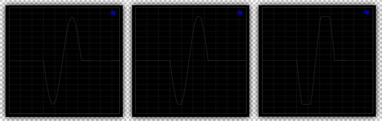
As covered earlier in the harmonic distortion section, higher order and increased levels of these harmonics could reshape a waveform into a virtual square wave. Clipping Distortion does exactly this, and it occurs when the input signal is high enough to drive the amplifier beyond its rated maximums. Clipping distortion adds odd-ordered upper harmonics to the signal, such as third, fifth, and seventh orders of harmonic distortion. While clipping should always be avoided during listening, the output section of an amp should be the first stage to clip. However, this has not always been the case. Sometimes, a preamplifier, or an earlier stage in a power amplifier will be asked to exceed its maximum capability before the successive current output stages. The result is that the power stage of the amplifier never reaches it full capability, thus hampering the headroom and dynamic capabilities during playback.
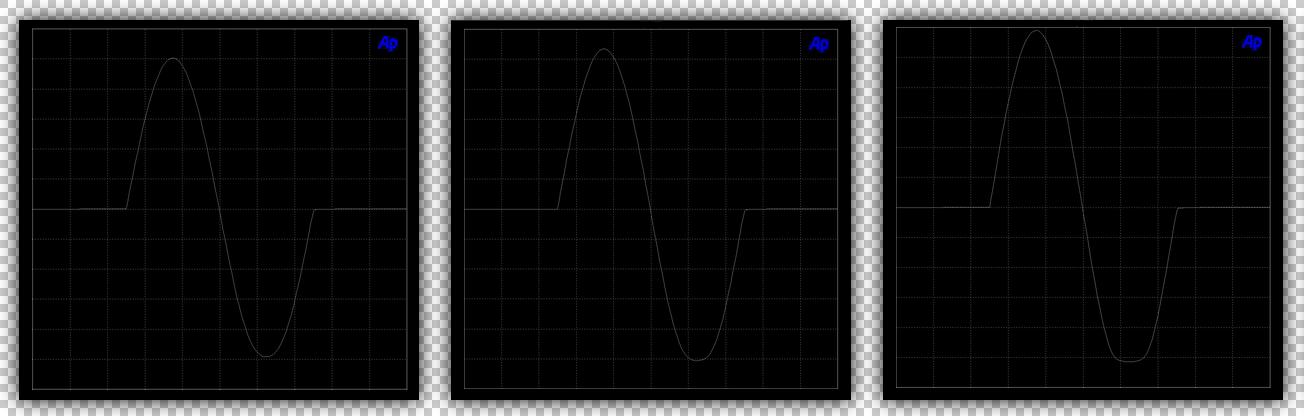
There are two major subcategories of clipping that are well deserved of mention here; voltage modulus threshold clipping, where the device under test can not reproduce a waveform greater than it’s specific maximum voltage, and the second; current clipping, where the voltage magnitude remains deformation free, but the current flow magnitude clips, thus failing to meet its sinusoidal goal and hampering the net Power delivery. Both of these are vastly different scenarios. However, because of the types of speakers that we use today, all production amplifiers are voltage-drive types instead of current amplifiers. They can supply current as a function of Ohms Law, but cannot drive it. Current drive amplifiers will not permit everyday loudspeakers to function properly unless they have been modified to suit such an amplifier.
Clipping Distortion can be dangerous to loudspeaker drivers. This is particularly important regarding tweeters and mid-range drivers, because these speaker cannot move to dissipate heat. Clipped crests carry several odd-ordered harmonics that are permitted past the speaker’s crossover network, raising the duty cycle. This leads to an-uncontrolled thermal rise and the overheating of the tinsel leads, copper or aluminum conductors, and the glue on the former. It should be avoided at all costs, and it can through giving proper attention to amplifier power, driver sensitivity, and impedance.
Amplitude Distortion
The name Amplitude Distortion bares some close resemblance to a previously discussed distortion, but this is its own classification. It has been characterized by a flattening of the 90, or 270 degree peaks of a waveform, but not both. Amplitude Distortion is demonstrated by an amplifying device exhibiting the capability to producing more power during one half of a waveform, but less during the other. This distortion invariably reduces the efficiency of a device, such as an amplifier. This is because the flattened crest of the waveform does nothing to contribute to the primary signal.
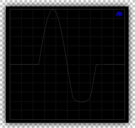
Semiconductors and thermionic valves have been characterized by a variety of parameters to make them predictable and user-friendly. Those values were used to decide where the devices were best suited, and how to construct the surrounding support circuitry to allow them to operate at their peak performance margins. One of those parameters was known as the transconductance curve. The curve relates to how the devices behave; where their maximum output lies when they were powered by a specific voltage and bias current, which would be regulated by the chosen componentry.
A flat, or constant linear curve has always been the goal of any good device, and sometimes designers chose devices that are less than optimal. Thermionic valves vary greatly from one model to another, and that made them suitible for a variety of tasks. One factor that remained quite constant, was that they displayed a relatively non-linear curve. In order to move the device into its most linear range for a given operating supply voltage and reduce distortion, they were biased considerably high. Some people have felt that placing the Q point far up into the positive side of the load line resulted in better sonic performance. It also allowed the device to supply current into the load when required. We see, in a signle ended design, the output current capability is determined by the bias current. However, current was not everything, as net Power (the quantity of Work being done) was formed by both the current and voltage potential. The problem faced with biasing the components too high, was that it introduced this non-linearity known as Amplitude Distortion.
In the case of biasing a single ended amplifier too high, the distortion occurs at the 90 and 270 degree peaks that breached the threshold of the positive supply voltage. Some Class A thermionic valve stages are overbiased, pushing the Q-point too far among the transconductance curve. The result, however, can give the impression of a an amplifier that has more drive and power headroom that it is really capable of.
In the case of a single-ended solid state device, if the bias was far too high, the positive half of the signal would saturate the device. This would result in the output decreasing to zero. Conversely, when a single-ended solid state amplifier’s bias was too small, the semiconductor could not fully conduct during the negative swings of the signal, and as a result the output would be set by the supply voltage. This is just like the thermionic valve amplifier example, above.
Class AB amplifiers have mostly been built using bipolar, or dual ended supplies out of practicality. This was because the actual output is recreated using a push-pull arrangement, where one half of the amplifier produces the positive swing potential of the waveform and the other produces the negative potential. While it is possible to build one with a single ended supply, there is little reason for the added complexity in creating a pseudo-neutral ground plane. Amongst the more common bipolar arrangements, the positive line was designated to powering the positive half, and a negative supply line fed the negative half.
If one of these supplies induced a voltage drop through current limiting, or other defects, it would not be able to supply equal quantities of energy to both the positive and negative halves of the output waveform. Just as was the case with single ended amplifier, one half of the audio waveform would prematurely clip. However, the major difference was that Amplitude Distortion and quiescent bias in Class AB designs were unrelated. Bias can be virtually any value in this topology without affecting the maximum output power, or clipping behavior, so long as the devices are in their linear range.
Dynamic Frequency Response Shift
Dynamic Frequency Response Shift is directly related to amplitude distortion, above. When the peaks of a complex waveform carry higher frequencies and these become clipped by inadequate headroom, two events take place. The higher frequency information which may be formed of vocals and instruments is greatly attenuated and sometimes even completely removed. As we know, clipping introduces new harmonic contributions. The removal, or reduction of higher frequency information combined with a new spectrum of odd-ordered harmonics produces a new sonic event that was never part of the original.
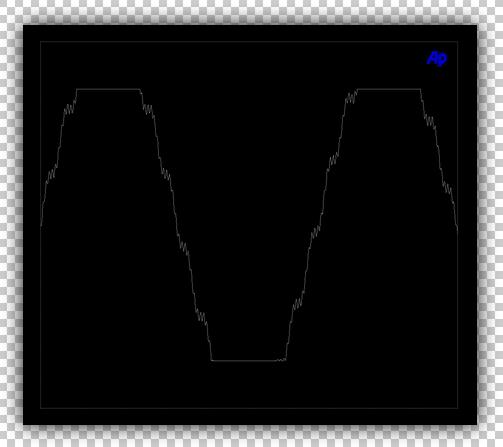
Because this type of distortion changes on a dynamic basis, usually leaving the bass line untouched, it may start out difficult to identify it as a problem inherent in the sound system rather than the recording, itself. In some cases, musical cues and components will appear to cut in and out of the programme, while the kick drums and bass rifts sound clean. Dynamic Frequency Response Shift can in some cases sound almost identical to aggressive dynamic compression, like that used in live performance venues.
Power
Oh yes, we love Power. Power is the relative quantity of Work that is capable of being completing within a specified time frame. Power output compared to the Power input provides an interface to gauge the effective efficiency of a device. Power output is most often found being represented in a unit measurement known as Wattage, a value which is the product of an electromotive force, called a Voltage, multiplied by a net sink of current flow, called Amperes. When a Voltage is applied to a resistive medium, a controlled rate of electron hole-flow occurs. The quantity of charge and energy transfer is measured in relation to time, as coulombs per second. The Voltage multiplied by the Amperes provides the information on the work being done as Watts. Voltage and current work in unison, and one without one the other becomes irrelevant since no work can done on their own. In this way they are largely inseparable.
There are two fundamental power ratings employed within the broad scope of audio electronics: Maximum Power measurements. which stand representative of the maximum work capability, and finally the Dynamic Audio Power (DAP), which concludes the power ratings. Both of these quantification are important and relay information about the device under test. In the case of an amplifier, they can provide knowledge of what it is capable of with some additional insight into the design methodology.
“Home theater and audiophile amplifiers are not regulated by the Federal Trade Commission and manufacturers are not required to meet any continuous Power standards.”
In controlled testing, Maximum Power is quantified with a continuous signal of while noise, spanning from just above DC to several hundreds of kilohertz. White noise is more demanding than a single tone, and the final numbers represent the maximum power of the amplifier. Depending on the manufacturer’s intentions, the test can last from five seconds to several days, without break.
Where home audio reproduction rarely sees the needs for continuous high-power reproduction, these tests are often brief. However, they must not be so short as to provide misleading numbers. A useful test must last longer than the time required for the power supply’s filter bank to charge continuously from the secondary windings of the power transformer(s) to provide relevant information.
Applications that require a specialized amplifier to perform under heavy duty cycles will be tested for extended periods. These are typically power amplifiers for noise control and professional use, and this challenging condition simulates a situation far more demanding than audio usage. Under testing circumstances, the amplifier is positioned as it is intended to be used and powered by a line Voltage that represents a nomal value in the real world. The amplifier is operated just below clipping and the output power is progressively reduced until the amplifier’s temperature stabilizes, thus ceasing to threaten thermal destruction from the impending overtime. The final value reflects the constant power output, along with some margin for safety.
The second rating, Dynamic Audio Power, is occasionally the subject of semantic confusion with Maximum Power. D.A.P is actually the measure of the amplifier’s headroom during the simultaneous reproduction of any number of frequencies, while connected to a shifting load impedance. Fewer products provide this data, because they are incapable of any noteworthy headroom. Dynamic Audio Power cannot be sustained, and relies upon the filter bank’s energy storage to support the peaks. Modern power amplifiers that are capable of dynamic headroom typically display traits of fast recovery, as the result of a well-made power transformer along with low output impedance.
Power Density is often represented by what we know as the Root Mean Squared, abbreviated as R.M.S. Root Mean Squared Power a misnomer for average power that can be referenced in comparison to an equivalent direct current value. Power is simply the product of the RMS Volts and RMS amps, and the resulting figure is Power in Watts. The term Root Mean Squared can only be applied to these two principle factors and not Power, itself. Maximum Power would invariably be equal to the RMS value by the nature of the very mathematics upon which they are each founded. The situation is underpinned by the fact that Root Mean Squared implies that if the magnitude of the cumulative sinusoidal waveform were to be summed into symmetrically square waves, which happen to coincidentally fall at .707 in relative magnitude, and were then rectified, the result would be a direct current providing the same thermal dissipation in BTU’s. Although they appear different, they hold the same Power Density, measured in Joules. The rating that we know as RMS Power is moreover a product of the earlier years in audio and only implies that the signal is based on RMS values. Please bare in mind that if a product’s Maximum Power is stated to be greater than the RMS value, then one of the values has been misrepresented.
The salient and underlying problems with Power ratings cannot be found within the progression of regulation, but rather the stasis wherein virtually none applies. Home theater and audiophile amplifiers are not regulated by the Federal Trade Commission and manufacturers are not required to meet any continuous Power standards. In a variety of cases, many very expensive audiophile amplifiers have shut down on the bench within seconds at less than half their rated output – forget about the low impedance tests. In contrast, some unsuspecting receivers and Japanese power amplifiers have been fully able to meet their rated specifications without incident. Adherence to any set method of testing is optional, and often verifying tests through third parties can be costly. As such, results vary exponentially, and it is hardly objective to compare home audio amplifiers by their power ratings. In light of this, several credible manufacturers have taken the time to provide IHF approved results for their products. If the Power rating provided complies with IHF standards, then the stated RMS Power should be interpreted as the Maximum Power rating. Products with ratings obtained through this method can be cross-examined within this lone context.
The purpose of an amplifier is to serve as a near-perfect voltage source, within reasonable limits. A perfect voltage source should be able to maintain a perfect voltage waveform, regardless of the load. However, the reality of the situation is that in order to support the signal voltage under load, the amplifier must also provide current when called upon to do so by the load. Most loads are not only resistive, but also reactive. At higher power levels, if the amplifier fails to provide ample current at frequencies where a loudspeakers requires such, it can induce a voltage drop. The declination in voltage magnitude manifests itself as the reduction in apparent amplitude, or sonic degradation. To keep ahead of the demand, the traditional amplifier must be foremost built upon a suitably capable power supply and output stage design.
High Current & Power Into Low Impedance Loads
Whenever the signal audio signal voltage and load resistance remains constant factors, current flow will also remain constant and unchanged. This is the fundamental foundation for the concept and application of Ohm’s Law, and it is unwavering. The largest majority of electrodynamic and electrostatic loudspeakers, however, are not purely resistive. Naturally, they are only resistive in one region and sometimes two or three additional portions of audio band with see resonance peaks, that are caused as associated components and enclosures, are introduced. As an alternating signal frequency is varied, the opposition to current flow decreases and increased at different frequencies. This condition arises where the current will be prone to latency and lag behind the voltage waveform, or the voltage will lead by a phase angle Theta. This is caused by the inductive and capacitive charge and discharge generating parameters of the load. This opposition and enticement to current flow is known as Impedance.
Provided that a reference frequency is available, impedance can be substituted into any mathematics expression that is based upon, or transposed from Ohm’s Law. Impedance can be the result of a series load that increases the apparent opposition to current flow, or an equivalent parallel shunt load that reduces the opposition. In either scenario, the impedance is subject to change with frequency. If the reactance occurs as a frequency-dependent shunt value, current flow increases in direct proportion to the reduction in impedance load. The cumulative impedance value represents the resistive portion of the load inclusive to the important effect brought by about the reactance.
High current is actually a misnomer for high feedback. This is because, before any amplifier can double its output current into a halved load impedance, it requires a satisfactory low output impedance to allow current to traverse the output devices.
Depending on the impedance to current flow from the service line, the amplifier’s power supply network, the output devices, cabling and all the way to the speaker’s motor assembly, there will be loss. This occurs whenever current flows through a conductive medium with resistance. In this way, higher current flow results in a lower efficiency and the loss is calculated as line drop. Line drop causes the voltage magnitude to decrease, which in turn introduces both linear domain and non-linear distortion. These effects correspond to a notable loss in amplitude at the frequencies that correspond to a region with a lower impedance. Another is harshness, or loss of perceived sound quality and detail as it becomes obscured by waveform deformation.
Impedance is very much among the more common misunderstood topics, but it is not some trivial nor pedantic distinction. Instead, understanding the difference between impedance an resistance is necessary to move toward any real understanding of electronic operation. As mentioned, it is the accumulation of the resistive element of a load and the reactive portion. Reactance may be capacitive or inductive, of which both are represented with the symbols Xc & Xl. The net value is modified by changing the frequency of an alternating current. The next time you see those symbols, you will have a better idea what they mean. The total Impedance for a given frequency can be stated as Z, and is commonly calculated as the product of the {square root of [R*2+[Xl-Xc]*2]}. While we are to do our best to avoid algebraic expressions here, there is importance in this simple and yet utmost important equation.
Inductance is not resistance, and rather, it is the frequency dependent dynamic opposition to change in current flow or a change in voltage magnitude through a conducting medium. As current flow increases, inductance tries to oppose this change. As current decreases, inductance tries to maintain current flow at it’s previous magnitude. Capacitance is the opposition to any change in voltage, and can be defined as the ability of an electrical device to store & release energy in an electrostatic field back onto a closed circuit. In the case of a loudspeaker, capacitive or inductive reactance occurs when the moving plane of a driver and its attached coil are moving at a different rate than the musical signal current, and a charge is generated and fed back on the output and power stage of the amplifier.
Since the voltage waveform from a device operates with the prime intent to remain unchanged regardless of load, it is the current that must change. If a loudspeaker exhibits a decrease in the numerical impedance value, current hole-flow is increased. If a loudspeaker load is very reactive and decreases from 7 down to 3.5 Ohms, twice as much current will attempt to traverse the load circuit. An audio power amplifier that doubles it’s current (and subsequent net output power) into a halved impedance load can provide a uniform clipping threshold over the entire frequency transfer range, and may offer good signal integrity at all frequencies. This is often casually regarded as high current. However, this is not always a prerequisite for satisfactory audio reproduction, as it is level and load dependent. In fact, should an amplifier fail to double its output power, the primary difference will be a three decibel reduction in maximum amplitude before the onset of clipping. It may distort more depending on its circuit design, or it very well may not. This is dependent on the science of the design.
High current has been a common topic among audio enthusiasts for a number of years. High current is actually a misnomer for high feedback. This is because, before any amplifier can double its output current into a halved load impedance it requires a satisfactory low output impedance to allow current to traverse the output devices.
The output design begins with the decision upon what kinds of loads the amplifier should drive, and what power it should have available to those loads. The output devices are then chosen to be rated higher than the current at that lowest impedance, and this ensures a long service life. These devices have a low “on” impedance, but not low enough. Increasing the instances of output devices can reduce the output impedance, but only by a small margin. The means by which to arrive at a low output impedance, which could then double current into 2 and 1 Ohms loads, is to apply a judicious degree of feedback around the output stage. With the output impedance sufficiently reduced as low as practical, the amplifier is then ready & reliant on its associated power supply to do the rest.
There are different approaches to providing higher currents on demand to the output devices, including but not limited to the conventional larger filter capacity banks, higher VA transformers, and even paralleled transformers. Each approach to power supply design is different and offers its own challenges and benefits, and before this paper arrives at that point some light will be cast on the topic. E-cores have the lowest output impedance and highest current capability, but often introduce higher noise. They can also be prone to mechanical vibration, by when sufficiently isolated they suffice as the prime means to high current. To reduce distortion, Faraday rings may be implemented into their design. R-cores have the highest output impedance but can offer vanishingly low harmonic noise and stray inductance, the result being a substantially large and costly transformer that offers a largely distortion-free sine wave. Carefully wound and shielded R-cores offer lower noise than rectifier blocks, themselves. A balance of cost and performance that has been common for many years is the toroidal transformer, which resides between the E and R core types. It is important that the transformer be adequate for the intended design and power expectations at various loads.
Where a transformer operates by converting a high voltage from the wall receptacle to a lower useable voltage, it functions based upon the principle of alternating current, abbreviated as A.C. Amplifiers and other electronics operate with direct currents, D.C, and thus the voltage must be rectified to such. A rectifier may be as simple as a monolithic device with four electrodes protruding from its package, of may be comprised of anywhere from two to eight discrete diodic devices. An audio component’s rectifier has a very important job and it is imperative that it can conduct with low noise, whilst withstanding the thermal stress induced by inrush hole-flow during the turn-on sequence and the high power levels that the amplifier is designed for.
The rectified direct current waveform retains the geometry of the original sinusoidal waveform from the electrical receptacle, but each half cycle now occurs in the same direction. Between the crests are valleys that must be smoothed and filled in an attempt to create a new continuous direct current. There are several ways to arrive at such conclusion, one being the use of a passive capacitance filter bank and the second being a filter bank in conjunction with active regulator circuitry.
Passive filter banks employ relatively large energy storage capacitors that charge when the rectified direct current pulses are near their crests and discharge during the time span residing between. Filter banks maybe comprised of a single large capacitor, to several hundred smaller value capacitors. What is important is that the equivalent series resistance be low enough it can also support the high power reproduction swings of the amplifier. The larger the capacitance, the greater the amount of work that it can do and the less residual A.C hum that will be present. The charging cycle is reliant on the ability of power transformer.
Most power amplifier output stages are supplied by passive and unregulated voltage rails. This alone constitutes partial reasoning for there being adequate filter supply capacitance affixed to the supply rails from the transformer(s) output. However, the size of the transformer(s) and filter capacitance are not accurate descriptors of the power amplifier’s sonic integrity, nor its cumulative output. This is not only because it relays zero information about the amplifier’s distortion traits, but also because some amplifying devices will perfectly double their output current until they reach the limit of the said margin of regulation. In this way, the maximum power ratings are still applicable, but where that amplifier may never be used near its maximums, it may perform substantially better than the numbers would otherwise suggest.
A power amplifier that produces a consistently measured output of, for example, four-hundred Watts with an intended supply voltage of 120 Volts, will not produce the same output if the line supply is reduced to 114 Volts. This remains a true performance factor, unless it is a regulated design. Active regulating and filtering typically entails the use of a power transformer which provide a higher voltage than what is required by the amplifier, or other device. The regulator induces a voltage drop to the desired potential while also referencing its output against its input to null the difference. The early preliminary stages of amplification should be regulated to maintain a constant voltage, for if they are not, the gain and headroom could be subject to change every time the service voltage fluctuated. When the design goal is applicable, actively regulated output stages are quite adept in their ability to double their output current, as needed. They can offer exemplary noise and hum levels, however, the cost often relegates active regulation to the preliminary driver stages alone in consumer audio and audiophile products.
When cost is an issue, regulated designs can be carried out in such manner that they double their output power into low impedance loads, thus providing high current on demand, to a predetermined point. The effectiveness is relative to this cost and complexity of the circuit, and where there is always a compromise based on monetary expenditures, the regulator eventually reaches a canyon wall in terms of power output into low impedance loads. The amplifier may even exhibit a decrease in power output into the lowest impedance. How much relevance this holds depends on the programme material, loudspeakers, and desired listening levels for the unspecified distance.
A very rare, expensive, and moreover complicated engineering approach to circumvent the undesirable characteristic of brick wall limiting entails a combination of regulation on a high energy core transformer, or two in parallel, and careful utilization of an isolated feedback network. Together they can supply a virtually perfect doubling into halved impedance loads with the highest voltage signal fidelity, without placing brick wall limitations above the regulator’s governing modes. This non-linear power curve gradually tapers and provides the sonic finesse of a much larger amplifier within its own intended range. The speaker’s load can be irrelevant down to one or two ohms, as far as the active power supply management is concerned. It also places no bars on the maximums, above which point it gradually begins to behave as a traditional amplifier. These amplifiers’ measure the same in IEC power rating tests as conventional amplifiers and may appear somewhat underwhelming at first glance, but make no mistake, as they offer musical and measured performance that is far more impressive below these ratings. There is great merit in this, because that is the intended power region where the amplifier will be used the most by the widest audience of customers.
“With just a few of these aspects briefly explained, many people can come to see how there is more to an amplifier than just net current reserve. It is the embodiment of how all other aspects of the device’s operation are important as well.”
While there is reason for certain listeners to choose satisfyingly high-power amplifiers that double their output power as impedance is halved, the fact remains that very few loudspeakers have a wide-band impedance that drops below three-Ohms. Adding to this, it is considered a poor engineering practice to do so.
In the case of electrostatics where a lower impedance has traditionally been more common, the lowest impedance magnitude traditionally resides in the highest frequency region where there is the least musical energy. It is common to hear that electrostatic loudspeakers are difficult to drive and that they require large amplifiers to survive low impedance loads. This myth is resilient, and to investigate this further requires some application of Ohm’s Law, the understanding of efficiency, and finally taking prudent account of the fundamental relationship between impedance and available net power.
Covered thus far, power amplifiers that are based on semiconductors have the ability to approximately double their output current, and power, each time the load impedance is reduced by half. Such an amplifier may provide one-hundred Watts of power into eight Ohms, two-hundred Watts into four Ohms, and four-hundred Watts into two Ohms. Should the design encompass the requisite provisions that sustain such, the amplifier may even double into one Ohm. However, this is all for naught with an electrostatic loudspeaker; the amplifier will only provide fifty Watts into sixteen Ohms, twenty-five Watts into thirty-two Ohms, and twelve and a half Watts into sixty-four Ohms.
Electrostatic loudspeakers are usually several times more inefficient that comparable electrodynamic loudspeakers, and thus require more power, ie Voltage and current, for similar playback levels. In an opposed fashion, electrostatic loudspeakers demonstrate a very high impedance which typically resides at the point of resonance in the bass registers, or, within the mid-range if a filter network is being utilized. For several notable designs, the impedance increases as a function of the input power squared. Pertinent to several electrostatic loudspeakers, the Q-factor at resonance lowers as power is increased, accentuating both the frequency coverage in addition to the magnitude of modulus. At resonance, the loudspeaker is largely non-reactive and mostly resistive. The low efficiency and high impedance to current flow introduces a scenario wherein there is very little power available over this frequency range. The result is that the power amplifier barely reaches a couple dozen Watts of output power at these bass frequencies when the protection & clipping circuits become active.
This is where specific thermionic valve amplifiers differ from their solid-state counterparts. An output transformer-less power amplifier may have 100 Watts available with an eight Ohms load, 90 Watts into four Ohms, and 55 Watts into two Ohms. Not very impressive on the low impedance side of the situation. Provided that the load impedance does not drop within the audible band, any reduction in the transfer magnitude can be mitigated to regions where it is largely regarded as inaudible. Here is the advantage of the output transformer-less thermionic valve amplifier – the power output is 100 Watts into sixteen Ohms, 97 Watts into thirty-two Ohms, and 95 Watts into sixty-four Ohms. This type of amplifier is chosen based upon the lowest impedance that it will have to drive and is designed specifically for it, while its available power into higher impedance loads remains very constant. This intermediate valve power amplifier will provide greater headroom when driving the identical electrostatic loudspeaker as the low-impedance high-current semiconductor type.
With just a few of these aspects briefly explained, many people can come to see how there is more to an amplifier than just net current reserve. It is the embodiment of how all other aspects of the device’s operation are important as well. Returning to the topic of power and high current, an amp that doubles it’s current into a halved impedance load will provide double the maximum output Power. It is the integral relationship between voltage and current that provide the power which determines the quantity of work that can be done. While particularly important with lower impedance and low efficiency electrodynamic loudspeakers, high current is often of reduced merit with the bulk of electrostatics.
To conclude this portion of the subject, an amplifier that does not double its apparent output current into a halved impedance will only have three decibels less headroom at the corresponding frequencies. The final decision on the type of power amplifier and its capabilities relies upon the desired playback levels and associated components which are to be used. Each component must not only work in a linear manner in its own right, but as a system. With all the adieu around current supply, it is good practice to keep in mind that if the first reigning voltage driver and any successive stages have been compromised by improper design practices, no quantity of current delivery capability will correct the distortion introduced during those steps in amplification.
Damping Factor
Damping Factor is a numeric expression that describes the relationship between a load impedance and the output impedance of a device. It is derived by dividing a specified load by the measured drive source impedance, with the the result representing the impedance to current hole-flow between the load and earth. A high Damping Factor indicates a low output impedance for supple current delivery, and the ability to shunt a foreign electromotive force when the signal changes, or ceases.
Damping has become a point of interest among audio enthusiasts, and in the context of certain loads it bares some limited importance. A loudspeaker driver has four fundamental mechanisms for motion control. They include the materials damping and geomatic architecture, secondly; the acoustical aspects of the air mass loading on the forward and rear surfaces of the driver diaphragm in combination with any compression inside the workings of the driver, thirdly; the mechanical aspect of the suspension and its compliance, and finally; the fourth being completion of the electrical circuit provided by the power amplifier. The moving mass of a driver’s radiating assembly accumulates kinetic energy in the form of inertia while it accelerates, causing the assembly to overshoot and continue in one direction. It does this only until the opposite force is great enough to cause it to decelerate at a sufficient rate and change direction.
All drivers, be them ribbons, planar, electrostatics and moving cone assemblies, each have mass. Matter, itself, is a property of mass structure. The result of the inherent mass, shape, and physical degree of motion is that they all exhibit energy storage behaviors to varying degrees, and at different frequencies. Overshoot during audio reproduction can occur even if the voltage waveform from the power amplifier calls for the driver to revert to a motion in the opposite direction. During the moment of overshoot, the voice coil within the magnetic gap acts as a microphone and generates an electromotive force, one that is not related to the audio signal. This is known as back-electromotive force, or back-E.M.F. It differs from the phase shift caused by driver non-linearites, because back E.M.F occurs at resonance points where the electrical aspect is resistive.
An amplifier with a lower output impedance has the ability to effectively shunt this voltage potential and can curtail any unwanted energy. However, the importance of damping factor criteria above one hundred may be all for naught in most audio systems. The effectiveness of this damping and overshoot attenuation is reliant upon the conductors, along any resistive elements in series with the load. The length of the cabling along can dwarf impedance of the amplifier and relegate the final effective damping to single digit values. Adding to this, loudspeakers that utilize common invasive passive crossovers will increase the series resistance, thus further reducing the amplifier’s effective damping. This, of course, negates the intended benefit of low frequency motion control near resonance.
Even so, it is a good practice to keep cable runs to adequate short lengths and to use the appropriate gauge of wire to prevent high frequency loss. Any additional damping is an added bonus and it costs nothing extra. On this topic, there is also an old audiophile myth that states if a listener inserts a resistor in series with woofer of a loudspeaker system, it will lower damping and raise Qts to reduce the low frequency articulation, control excursion, and provide a sound closer to that of a thermionic valve design. This story is unfortunately based upon the misunderstanding of the electromechanical principles of driver operation. This is easily demonstrated, as any theoretical gains realized by a higher total system resonance Q-factor occur at the expense of insertion loss and a raised electrical compliance. The addition of a series resistive medium leads to an increased mechanic Q through an unwanted increase in the electrical compliance measurement, as opposed to increasing mechanical compliance alone, thus negating the origin intent.
When an amplifier provides better low frequency information and coincidentally has high damping factor, most of the improvements can be traced back to the use of feedback, providing improved waveform linearity. The equivalent shunt resistance of an amplifier is in the order of several magnitudes lower and damping capabilities higher among solid state designs than vacuum tube designs. While it can be improved further in amplifiers facilitated with paralleled output stages, any possible damping from a low output impedance should perhaps never be solely relied upon as the means of compensation, for what should have been prime consideration during the design stages of the loudspeakers.
Summary & Conclusion
In closing, designing high performance audio equipment really is much like any of scientific endeavor – there is as much trigonometry, algebra and calculus compounded by as many variables involved during the design of a quality audio system as there is in sending a missile one-hundred miles to a test designation. After all the work has been done, it is still the sound that matters most.
I hope that readers enjoyed this segment and that they perhaps took something useful from amongst the many valuable points that have been shared here, today. Maybe it helped clarify something about that amplifier you are working on, or sparks a fresh and creative idea for a project. Maybe it will even help with that next audio component purchase. In any case, I hope that this casual paper not only educates, but also stimulates further progress and creativity among readers. I wish each and everyone out there many happy hours enjoying your favorite music.
[views]
I did not find any distortions related to the signal propagation delay in the article. Distortions related to the signal deviation from a stationary sinusoid (at the moments of amplitude change, at the moments of frequency change, with simultaneous change of both parameters) are also not reflected. Distortions related to the rotation of the signal fronts (slopes) that occur in linearly increasing/decreasing sinusoids, with the sum of two signals, in amplitude-modulated signals are not reflected.
Best regards,
Alexander Petrov